We have discussed how to describe the quantum evolution of open quantum systems and we have introduced the concept of dynamical map $\Lambda_t$ and its time-dependent generator $L_t$. The latter quantity is also known as the dissipator and describes the form of the master equation. The connection between the two is given by Eq. (2.29). A very important problem in the theory of open quantum systems is the following:

Problem 1

What are the properties of the local time-dependent generator $L_t$ that guarantee $\Lambda_t$, as defined by the T-product exponential formula (2.29), defines a legitimate dynamical map?

The formulation of our problem is pretty simple, but in general the answer is not known. In fact, it turns out that the answer is only known for the special case of time-independent generators, giving rise to Markovian semigroups. In this case the answer to this important problem is given by the GKSL theorem discussed in Chapter 4. But what about more general types of generators?

Let us observe that if we knew a dynamical map $\Lambda_t$ that was invertible, i.e. there exists $\Lambda_t^{-1} : \Mn \ra \Mn$ such that $\Lambda_t^{-1} \Lambda_t = \Lambda_t \Lambda_t^{-1} = \mathbb{1}_n$, then

\begin{equation} \dot{\Lambda}_t = \dot{\Lambda}_t \Lambda_t^{-1} \Lambda_t = L_t \, \Lambda_t\ , \tag{5.1} \end{equation}

where we defined \begin{equation} L_t := \dot{\Lambda}_t \Lambda_t^{-1} \ . \tag{5.2} \end{equation}

It should be stressed that the inverse of $\Lambda_t$ need not be CP. One may prove that if $\Lambda_t$ is CP then $\Lambda_t^{-1}$ is CP if and only if $\Lambda_t(\rho) = U_t \rho U_t^\dagger$ with unitary $U_t$.

Example 6

Consider a unitary dynamical map $\mathcal{U}_t$ defined in (2.23). It is clear that $\mathcal{U}_t$ is invertible and $\mathcal{U}_t^{-1} = \mathcal{U}_{-t}$ is CP. One finds for the corresponding generator \begin{equation} L_t(\rho) = [\dot{\mathcal{U} }_t \mathcal{U}_{-t}](\rho) = \dot{U}_t (U_t^\dagger \rho U_t) U_t^\dagger + {U}_t (U_t^\dagger \rho U_t) \dot{U}_t^\dagger \ , \tag{5.3} \end{equation}

and hence recalling that $U_t$ satisfies the Schrödinger equation $\dot{U}_t = -iHU_t$, one obtains $L_t(\rho) = -i[H,\rho]$.

In this course instead of analyzing this problem in full generality we restrict ourselves to study special classes of dynamical maps and corresponding local generators. Specifically we analyze 3 important classes of generators

• $C_1$ - a class of time-independent generators giving rise to Markovian semigroups,
• $C_2 $ - a class of time-dependent generators giving rise to commutative dynamics,
• $C_3 $ - a class of time-dependent generators giving rise to the so-called divisible dynamical maps.

5.1. Commutative dynamics

We call a dynamical map $\Lambda_t$ commutative if $[\Lambda_t,\Lambda_u]=0$ for all $t,u\geq 0$. It means that for each $A\in \Mn$ one has

\begin{equation} \Lambda_t(\Lambda_u(A)) = \Lambda_u(\Lambda_t(A)) \ . \tag{5.4} \end{equation}

It is easy to show that commutativity of $\Lambda_t$ is equivalent to commutativity of the local generator

\begin{equation}\label{[]=0} [L_t,L_u]=0\ , \tag{5.5} \end{equation}

for any $t,u \geq 0$. Note that in this case the formula (2.30) considerably simplifies: the 'T' product drops out and the solution is fully controlled by the integral $\int_0^t L_u du$: \begin{equation}\label{Dyson-com} \Lambda_t = \exp\left( \int_0^t L_u du\right) = \mathbb{1}_n + \int_0^t L_{u}du + \frac 12 \left( \int_0^{t} L_{u}du \right)^2 + \ldots \ . \tag{5.6} \end{equation}

Now, it follows from Theorem 3 that if $\Lambda = e^M$, then $\Lambda$ is a quantum channel if $M$ is a GKSL generator. Therefore, one has the following

Theorem 4

If $L_t$ satisfies (\ref{[]=0}), then $L_t$ is a legitimate generator if $\int_0^t L_\tau d\tau$ is a GKSL generator for all $t\geq 0$.

Note that, if $L_t = L$ is time independent, then $\int_0^t L_udu = tL$ and the above theorem reproduces Theorem 3.

It is clear that if $L$ is a legitimate GKSL generator and $f: \mathbb{R}_+ \ra \mathbb{R}$ an arbitrary function, then $L_t = f(t) L$ generates a commutative dynamical map $\Lambda_t$ iff $\int_0^t f(u) du \geq 0$ for all $t\geq 0$. A typical example of commutative dynamics is provided by

\begin{equation} L_t = \omega(t) L_0 + a_1(t) L_1 + \ldots + a_N(t) L_N\ , \tag{5.7} \end{equation}

where $[L_\alpha,L_\beta]=0$ with $L_0(\rho) = -i[H,\rho]$, and for $\alpha>0$ the generators $L_\alpha$ are purely dephasing, that is, $L_\alpha(\rho) = \Phi_\alpha(\rho) - \frac 12 \{ \Phi_\alpha^*(\mathbb{I}),\rho\}$. One has for the corresponding dynamical map

\begin{equation} \Lambda_t = e^{\Omega(t)L_0} \cdot e^{A_1(t)L_1} \cdot \ldots\cdot e^{A_N(t)L_N}\ , \tag{5.8} \end{equation}

with $$ \Omega(t) = \int_0^t \omega(u)du\ ; \ \ \ \ A_\alpha(t) = \int_0^t a_\alpha(u)du\ . $$

It is clear that $\Lambda_t$ is CP iff $A_\alpha(t) \geq 0$ for all $\alpha=1,\ldots,N$.

Example 7

Consider a qubit generator $L_0(\rho) = -i[\sigma_3,\rho]$ together with $L_1,L_2,L_3$ defined in (5.27). One easily proves

\begin{equation} [L_0,L_\alpha] = [L_3,L_\alpha]=0 \ ; \ \ \ \alpha=1,2,3\ , \tag{5.9} \end{equation}

and \begin{equation}\label{L-L} [L_1,L_2] = L_1 - L_2 \ . \tag{5.10} \end{equation}

Define the time-dependent commutative generator

\begin{equation} L_t = \frac{\omega(t)}{2} L_0 + \frac{\delta(t)}{2} ( \mu_1 L_1 + \mu_2 L_2) + \frac{\gamma(t)}{2} L_z\ , \tag{5.11} \end{equation}

with $\mu_1,\mu_2 \geq 0$ and $\mu_1 + \mu_2=1$. Defining

\begin{equation} \Omega(t) = \int_0^t \omega(u)du\ ; \ \ \Delta(t) = \int_0^t \delta(u)du\ ; \ \ \Gamma(t) = \int_0^t \gamma(u)du\ , \tag{5.12} \end{equation}

one finds that if $\Delta(t) \geq 0$ and $\Gamma(t) \geq 0$, then $L_t$ is a legitimate generator. The time evolution of $\rho$ has the following form: the off-diagonal elements evolve according to

$$\rho_{12} \ra e^{\Omega(t) + \frac 12 \Delta(t) + \Gamma(t)} \rho_{12}\ , $$

and diagonal elements

\begin{eqnarray*} \rho_{11} &\ra & \rho_{11}\, e^{-\Delta(t)} + \mu_1 \Big[ 1 - e^{-\Delta(t)} \Big] \ ,\\ \rho_{22} &\ra & \rho_{22}\, e^{-\Delta(t)} + \mu_2 \Big[ 1 - e^{-\Delta(t)} \Big] \ . \end{eqnarray*}

If $\Delta(t) \ra \infty$ for $t\ra \infty$, then the dynamics possess an equilibrium state

$$ \rho_t \ \ \longrightarrow \ \ \left( \begin{array}{cc} \mu_1 & 0 \\ 0 & \mu_2 \end{array} \right) \ . $$

Example 8 (Random unitary qubit dynamics)

Consider the following time-dependent generator \begin{equation}\label{Pauli} L_t(\rho) = \frac 12 \sum_{k=1}^3 \gamma_k(t) (\sigma_k \rho\, \sigma_k - \rho)\ , \tag{5.13} \end{equation}

where $\{\sigma_1,\sigma_2,\sigma_3\}$ are Pauli matrices. It is easy to prove that $[L_t,L_u]=0$ and hence $L_t$ generates a legitimate dynamical map iff

$$ \Gamma_1(t) \geq 0 \ ; \ \ \Gamma_2(t) \geq 0 \ ; \ \ \Gamma_3(t) \geq 0 \ , $$

where $\Gamma_k(t) = \int_0^t \gamma_k(u)du$. One finds that the corresponding dynamical map $\Lambda_t$ is given by

\begin{equation}\label{RU} \Lambda_t(\rho) = \sum_{\alpha=0}^3 p_\alpha(t) \sigma_\alpha \rho\, \sigma_\alpha \ , \tag{5.14} \end{equation}

where $\sigma_0 = \mathbb{I}_2$ and

\begin{eqnarray*} p_0(t) &=&\frac{1}{4}\, [1+ \lambda_3(t) + \lambda_2(t) + \lambda_1(t)] \ , \\ p_1(t) &=&\frac{1}{4}\, [1- \lambda_3(t) - \lambda_2(t) + \lambda_1(t)] \ ,\\ p_2(t) &=&\frac{1}{4}\, [1- \lambda_3(t) + \lambda_2(t) - \lambda_1(t)] \ ,\\ p_3(t) &=&\frac{1}{4}\, [1+ \lambda_3(t) - \lambda_2(t) - \lambda_1(t)] \ , \end{eqnarray*}

with $$ \lambda_1(t) = e^{-\Gamma_2(t) - \Gamma_3(t)}\ , $$

and similarly for $\lambda_2(t)$ and $\lambda_3(t)$. Interestingly $\Lambda_t(\sigma_k)=\lambda_k(t)\sigma_k$. The formula (\ref{RU}) defines so-called random unitary dynamics. Note that

$$ p_0(t) + p_1(t) + p_2(t) + p_3(t)=1 \ . $$

Moreover, $p_\alpha(t) \geq 0$ for $\alpha=0,1,2,3$ iff $\Gamma_k(t) \geq 0$ for $k=1,2,3$. Note that $\Lambda_t$ is unital. Actually, in the case of qubits any unital dynamical map is random unitary, i.e.

\begin{equation}\label{} \Lambda_t(\rho) = \sum_k p_k(t) U_k(t) \rho U_k^\dagger(t)\ , \tag{5.15} \end{equation}

where $p_k(t)$ defines time-dependent probability distribution and $U_k(t)$ is a family of time-dependent unitary matrices. It is no longer true for $n$-level systems with $n>2$.

IBM Q example: Pauli channel

The most general single-qubit open quantum system model is the time-dependent Pauli channel. The master equation in this case takes the form (see Eq. (\ref{Pauli}))

\begin{equation} \frac{d\rho_{S} }{dt}(t)=\frac{1}{2}\sum_i\gamma_i(t)\left[\sigma_i\rho_{S}(t)\sigma_i-\rho_{S}(t)\right]. \label{PauliME} \end{equation}

Generally, the dynamics described by the master equation above is not phase-covariant [1], except for the case in which $\gamma_x(t)=\gamma_y(t)$. Moreover, since the decay rates may take negative values, conditions for complete positivity must be imposed, and they are given in terms of a set of inequalities involving all the three decay rates, as one can see, e.g., from Ref. [2].

At a specific time instant $t$, the Pauli channel can be written as \begin{equation} \mathcal{E} (\rho) = \sum_{i=0}^3 p_i \sigma_i \rho \sigma_i, \end{equation}

with $0 \leq p_i \leq 1$ and $\sum_i p_i = 1$. The depolarizing channel is a special case of the Pauli channel where $p_1 = p_2 = p_3 = p/4$.

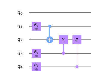
It is possible to implement the general Pauli channel with just two ancillary qubits, by preparing them in the suitable entangled state. The first qubit acts as the control for a controlled-$X$ (CNOT) gate, and the second one for a controlled-$Y$. Notice that applying both an X and a Y gates is effectively equivalent to applying a Z gate.

The state $|\psi \rangle$ of the ancillae needed for the Pauli channel can be implemented by the following circuit:

The circuit is parametrised by the three angles $\theta_1,\theta_2,\theta_3$. The state of the two ancillae is as follows: \begin{equation*} \begin{split} | \psi \rangle =& (c_1 c_2 c_3 + s_1 s_2 s_3) | 00 \rangle + \\ & (c_1 c_2 s_3 - s_1 s_2 c_3) | 01 \rangle + \\ & (c_1 s_2 c_3 - s_1 c_2 s_3) | 10 \rangle + \\ & (s_1 c_2 c_3 + c_1 s_2 s_3) | 11 \rangle \end{split} \end{equation*}

where $c_i \equiv \cos \theta_i$ and $s_i \equiv \sin \theta_i$.

The angles $\theta_i$ can be found by solving the following system of equations:

\begin{equation}\label{eq:pauli_equations} \begin{cases} p_0 = |\langle 00|\psi \rangle|^2 = (c_1 c_2 c_3 + s_1 s_2 s_3)^2 & \\ p_1 = |\langle 01|\psi \rangle|^2 = (c_1 c_2 s_3 - s_1 s_2 c_3)^2 & \\ p_2 = |\langle 10|\psi \rangle|^2 = (c_1 s_2 c_3 - s_1 c_2 s_3)^2 & \\ p_3 = |\langle 11|\psi \rangle|^2 = (s_1 c_2 c_3 + c_1 s_2 s_3)^2 & \end{cases} \end{equation}

The above system of equations allows for multiple analytical solutions whose expressions are too cumbersome to be reported here. The choice of the solution to use in each case depends on a number of factors, such as the gate fidelity for the specific values of the parameters.

IBM Q Example: Depolarizing channel

The depolarizing channel is one of the most common models of qubit decoherence due to its nice symmetry properties. We can describe it by stating that, with probability $p$ the qubit remains intact, while with probability $1-p$ an error occurs. The error can be a bit flip error, described by the action of $\sigma_x$, a phase flip error, described by the action of $\sigma_z$, or both, described by the action of $\sigma_y$. The dynamical map of a Markovian open quantum system subjected to depolarizing noise can be written as

\begin{eqnarray}\label{depolarising_channel} \Phi_t \rho_S = \left[1-\frac 3 4 p(t)\right] \rho_S + \frac{p(t)}{4} \sum_i \sigma_i \rho_S \sigma_i, \end{eqnarray}

where $i=x,y,z$ and $p(t)=1 - e^{-\gamma t}$, with $\gamma$ the Markovian decay rate.

Please note that in Pauli channel example for $\gamma_i(t) = \gamma$, we recover the Markovian depolarizing channel.

The depolarizing channel can be implemented, for any value of $p\equiv p(t) \in [0, 1]$, with the circuit shown in the figure above. Three ancillary qubits are prepared in a state $| \psi_\theta \rangle = \cos \theta/2 | 0 \rangle + \sin \theta/2 | 1 \rangle$, and are used as controls for, respectively, a controlled-$X$ (CNOT), a controlled-$Y$ and a controlled-$Z$ rotation. This way, each gate will be applied with a probability $\sin^2 \theta/2$.

The rotation angle $\theta$ must be chosen so that each of the gates is applied with probability $p$. Notice that applying $X$ and then $Y$, but not applying $Z$ is equivalent (up to global phases) to just applying $Z$, and so on. The resulting equation that binds $\theta$ to $p$ is thus

\begin{equation} \sin^2 \frac \theta 2 \cos^4\frac\theta2 + \sin^4 \frac\theta 2 \cos^2 \frac \theta 2 = \frac p 4, \end{equation}

with solution $\theta(p) = \frac 12 \arccos(1 - 2 p)$.

Notice that the circuit for the Pauli channel can be used also for the depolarizing channel, instead of the three-qubit circuit of the figure above, but it proves to be less accurate on the IBM Q Experience devices, presumably because of the required entanglement between the two qubits.

One could also think to implement the Pauli channel by generalising the depolarizing channel circuit, specifically, by allowing for the three ancillae to be prepared in different states. One can see, however, that this cannot be done in the most general case.

Figure 1. Density matrix elements of a qubit affected by a depolarizing channel for different values of the parameter $p$. Points correspond to the experimental tomographic reconstruction, while dashed lines show the theoretical prediction.

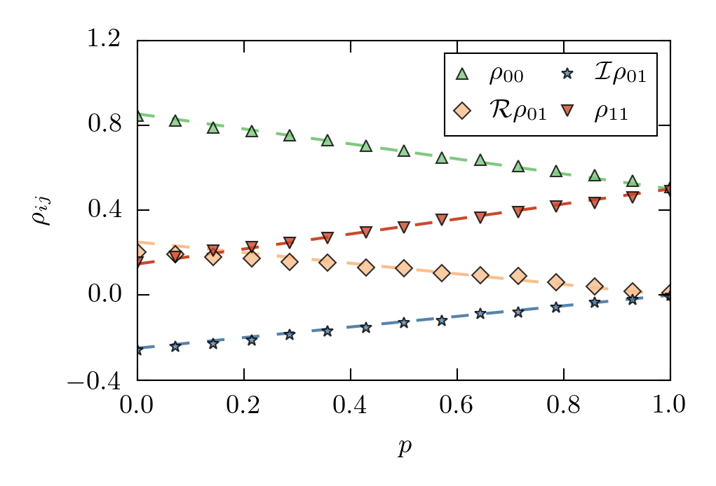
In Figure 1, we plot the qubit density matrix elements for various values of $p$, comparing the experimental data with the theoretical prediction. For exemplary purposes, we choose a specific initial state possessing non-zero coherences.

5.2. Markovian evolution - divisible dynamical maps

We call a dynamical map $\Lambda_t$ divisible if for any $t \geq s \geq 0$ one has the following decomposition

\begin{equation} \Lambda_t = V_{t,s}\, \Lambda_s \ , \tag{5.16} \end{equation}

with a completely positive propagator $V_{t,s}$. Note, that if $\Lambda_t$ is invertible then

\begin{equation} V_{t,s} = \Lambda_t \, \Lambda_s^{-1} \ , \tag{5.17} \end{equation}

and hence $V_{t,s}$ satisfies an inhomogeneous composition law

\begin{equation} V_{t,s} V_{s,u} = V_{t,u}\ , \tag{5.18} \end{equation}

for any $t\geq s \geq u$.

The above formula provides a generalization of the semi-group composition law (4.2). Here we assume the following extended definition of Markovian evolution: a dynamical map $\Lambda_t$ corresponds to Markovian evolution if and only if it is divisible.

Interestingly, the property of being Markovian (or divisible) is fully characterized in terms of the local generator $L_t$. Note, that if $\Lambda_t$ satisfies (2.28) then $V_{t,s}$ satisfies \begin{equation}\label{Local-V} \frac{d}{dt}\, V_{t,s} = L_t V_{t,s}\ , \ \ \ V_{s,s}=\mathbb{1}\ , \tag{5.19} \end{equation}

and the corresponding solution reads \begin{equation} V_{t,s} = {\rm T} \, \exp\left( \int_s^t L_u du \right)\ . \tag{5.20} \end{equation}

It is clear that $\Lambda_t = V_{t,0}$ which shows that divisibility puts very strong requirements upon the dynamical map $\Lambda_t$.

One proves the following

Theorem 5

The map $\Lambda_t$ is divisible if and only if $L_t$ is a GKSL generator for all $t$, that is,

\begin{equation} L_t(\rho) = -i[H(t),\rho] + \frac 12 \sum_k \left( [V_k(t),\rho V^\dagger_k(t)] + [V_k(t)\rho,V^\dagger_k(t)] \right) \ , \tag{5.21} \end{equation}

with time-dependent Hamiltonian $H(t)$ and noise operators $V_k(t)$.

Remark 3

If \begin{equation} L_t = \omega(t) L_0 + a_1(t) L_1 + \ldots + a_N(t) L_N\ , \tag{5.22} \end{equation}

where $L_0(\rho) = -i[H,\rho]$, and for $\alpha>0$ the generators $L_\alpha$ are purely dissipative and linearly independent, then $L_t$ generates Markovian evolution if and only if $a_1(t),\ldots,a_N(t) \geq 0$.

Example 9

Consider a qubit generator \begin{equation} L_t(\rho) = \frac 12 {\gamma(t)} L_3(\rho) = \frac 12 {\gamma(t)} (\sigma_z \rho \sigma_z - \rho)\ , \tag{5.23} \end{equation}

and introduce $ \Gamma(t) = \int_0^t \gamma(\tau)d\tau$, then it is clear that

\begin{equation} \Lambda_t(\rho) = \frac 12 \Big[ 1+ e^{-\Gamma(t)} \Big]\, \rho + \frac 12 \Big[ 1- e^{-\Gamma(t)} \Big]\, \sigma_z \rho \sigma_z\ , \tag{5.24} \end{equation}

and hence

1. $L_t$ is a legitimate generator iff $\,\Gamma(t)\geq 0$,
2. $L_t$ generates Markovian evolution iff $\gamma(t) \geq 0$,
3. $L_t$ generates a Markovian semigroup iff $\gamma(t) = {\rm const.} >0$.

Example 10

Let us consider a qubit generator defined by $H = \frac \omega 2 \sigma_z$ and the following CP map

\begin{equation} \Phi(\rho) = \gamma_1 \sigma_+ \rho\, \sigma_- + \gamma_2 \sigma_- \rho\,\sigma_+ + \gamma \sigma_z \rho\, \sigma_z\ , \tag{5.25} \end{equation}

where $\sigma_+ = |2 \rangle \langle 1|$ and $\sigma_-=|1 \rangle \langle 2|=\sigma_+^\dagger$ are standard qubit raising and lowering operators. The corresponding generator reads $L(\rho) = - i[H,\rho] + L_D(\rho)$ with the dissipative part

\begin{equation} L_D = \frac{\gamma_1}{2} L_1 + \frac{\gamma_2}{2} L_2 + \frac{\gamma}{2} L_z\ , \tag{5.26} \end{equation}

where \begin{eqnarray} \label{LLL} L_1(\rho) &=& [\sigma_+, \rho\sigma_-] + [\sigma_+ \rho, \sigma_-] \ ,\nonumber \\ L_2(\rho) &=& [\sigma_-, \rho\sigma_+] + [\sigma_- \rho,\sigma_+] \ , \\ L_3(\rho) &=& \sigma_z \rho\sigma_z - \rho \ . \nonumber \tag{5.27} \end{eqnarray}

$L_1$ corresponds to pumping (heating) process, $L_2$ corresponds to relaxation (cooling), and $L_3$ is responsible for pure decoherence. To solve the master equation $\dot{\rho}_t = L\rho_t$ let us parameterize $\rho_t$ as follows

\begin{equation} \rho_t = p_1(t) P_1 + p_2(t) P_2 + \alpha(t) \sigma_+ + \overline{\alpha(t)} \sigma_-\ , \tag{5.28} \end{equation}

with $P_k=|k \rangle \langle k|$. Using the following relations

\begin{eqnarray*} L(P_1) &=& {\gamma_1} (P_2 - P_1) = - \gamma_1\, \sigma_3\ , \\ L(P_2) &=& {\gamma_2} (P_1 - P_2) = \gamma_2\, \sigma_3 \ , \\ L(\sigma_+) &=& (i \omega - \eta)\, \sigma_+\ ,\\ L(\sigma_-) &=& (-i\omega - \eta)\, \sigma_-\ , \end{eqnarray*}

where one finds the following Pauli master equations for the probability distribution $(p_1(t),p_2(t))$

\begin{eqnarray} \dot{p}_1(t) &= &- \gamma_1\, p_1(t) + \gamma_2\, p_2(t) \ , \tag{5.29} \end{eqnarray}\begin{eqnarray} \dot{p}_2(t) &= & \ \ \, \gamma_1\, p_1(t) - \gamma_2\, p_2(t) \ , \tag{5.30} \end{eqnarray}

together with $\alpha(t) = e^{(i \omega - \eta)t}\alpha(0)$. The corresponding solution reads

\begin{eqnarray} p_1(t) &=& p_1(0)\, e^{-( \gamma_1 + \gamma_2)t} + p_1^* \Big[ 1 - e^{-( \gamma_1 + \gamma_1)t} \Big] \ , \tag{5.31} \end{eqnarray}\begin{eqnarray} p_2(t) &=& p_2(0)\, e^{-( \gamma_1 + \gamma_2)t} + p_2^* \Big[ 1 - e^{-( \gamma_2 + \gamma_2)t} \Big] \ , \tag{5.32} \end{eqnarray}

where we introduced

\begin{equation}\label{p*} p_1^* = \frac{\gamma_1}{\gamma_1 + \gamma_2}\ , \ \ \ \ p_2^* = \frac{\gamma_2}{\gamma_1 + \gamma_2}\ . \tag{5.33} \end{equation}

Hence, we have purely classical evolution of the probability vector $(p_1(t),p_2(t))$ on the diagonal of $\rho_t$ and very simple evolution of the off-diagonal element $\alpha(t)$. Note that asymptotically one obtains a completely decohered density operator

$$ \rho_t \ \ \longrightarrow \ \ \left( \begin{array}{cc} p_1^* & 0 \\ 0 & p_2^* \end{array} \right) \ . $$

In particular if $\gamma_1=\gamma_2$ a state $\rho_t$ relaxes to the maximally mixed state (a state becomes completely depolarized).

IBM Q example: Markovian reservoir engineering

Theory

For decades, noise induced by the environment has been considered the archetype enemy of quantum technologies. This is because very often the interaction between a quantum system and its surroundings leads to the fast disappearance of quantum properties, notoriously coherences and entanglement, playing a key role in providing quantum advantage. This point of view drastically changed as soon as physicists demonstrated that appropriate manipulation of an artificial environment (quantum reservoir engineering) would allow one to steer the open system towards, e.g., a maximally entangled state [3,4], hence turning upside down the perspective of the environment as an enemy.

Following the lines of Ref. [3], we experimentally simulate a semigroup Markovian master equation for a two-qubit open system having as asymptotic stationary state the Bell state $|\psi^- \rangle = \frac{1}{\sqrt{2} }(|01\rangle - |10\rangle)$, where we indicate with $|0\rangle$ and $|1\rangle$ the computational basis of each qubit and we use the notation $| 01\rangle = |0\rangle_1 |1\rangle _2$. This allows us to prepare a maximally entangled state as a result of the dissipative open system dynamics.

The four Bell states are:

\begin{align} |\psi^- \rangle = \frac{1}{\sqrt{2} }(|01\rangle - |10\rangle) \\ |\psi^+ \rangle = \frac{1}{\sqrt{2} }(|01\rangle + |10\rangle) \\ |\phi^- \rangle = \frac{1}{\sqrt{2} }(|00\rangle - |11\rangle) \\ |\phi^+ \rangle = \frac{1}{\sqrt{2} }(|00\rangle + |11\rangle) \end{align}

Each of them is uniquely determined as an eigenstate with eigenvalues $\pm1$ with respect to $\sigma_z^{(1)} \otimes \sigma_z^{(2)}$ and $\sigma_x^{(1)}\otimes\sigma_x^{(2)}$, where $\sigma_x^{(i)}$ and $\sigma_z^{(i)}$, with $i=1,2$, are the $x$ and $z$ Pauli operators of qubit 1 and 2.

The dissipative dynamics that pumps two qubits from an arbitrary initial state into the Bell state $|\psi^- \rangle $ is realised by the composition of two channels that pump from the $+1$ into the $-1$ eigenspaces of the stabiliser operators $\sigma_z^{(1)} \otimes \sigma_z^{(2)}$ and $\sigma_x^{(1)} \otimes \sigma_x^{(2)}$.

Specifically, we consider the two $p$-parametrised families of CPTP maps $\Phi_{zz} \rho_S = E_{1z} \rho_S E_{1z}^{\dagger} + E_{2z} \rho_S E_{2z}^{\dagger} $, with

\begin{equation}\label{KrausZZ} \begin{aligned} E_{1z} &=\sqrt{p} \mathbb{I}^{(1)} \otimes \sigma_x^{(2)} \frac{1}{2}\left( \mathbb{I}+ \sigma_z^{(1)} \otimes \sigma_z^{(2)} \right), \\ E_{2z} &= \frac{1}{2} \left( \mathbb{I}-\sigma_z^{(1)}\otimes\sigma_z^{(2)} \right) \\ &+ \sqrt{1-p} \frac{1}{2} \left( \mathbb{I}+ \sigma_z^{(1)}\otimes\sigma_z^{(2)} \right), \end{aligned} \end{equation}

and $\Phi_{xx}\rho_S = E_{1x} \rho_S E_{1x}^{\dagger} + E_{2x} \rho_S E_{2x}^{\dagger} $, where $E_{1x}$ and $E_{2x}$ have the same form of $E_{1z}$ and $E_{2z}$ in equations, provided that we replace $\sigma_x^{(2)}$ with $\sigma_z^{(2)}$ and $\sigma_z^{(1)}\otimes\sigma_z^{(2)}$ with $\sigma_x^{(1)}\otimes\sigma_x^{(2)}$.

By changing the parameter $0 \le p \le 1$ we simulate different types of open quantum system dynamics. For $p\ll1$, the repeated application of, e.g., $\Phi_{zz}$ generates a master equation of Lindblad form with jump operator $V=\frac{1}{2} \mathbb{I}^{(1)}\otimes\sigma_x^{(2)}\left( \mathbb{I}+ \sigma_z^{(1)} \otimes \sigma_z^{(2)} \right)$. For $p=1$, the map $\Phi_{xx} \circ \Phi_{zz}$ generates $|\psi_- \rangle $ for any initial state.

Circuit implementation

In Ref. [3], the authors provide the circuits for the implementation of the Bell-state pumping. However, these are composed of gates that are natural to the trapped-ions platform used in that work, so their direct implementation on the IBM Q Experience devices would result in far too long circuits. Therefore, we propose a different set of circuits that follow the same basic working principles, but have been designed specifically keeping in mind the characteristics of the IBM Q Experience platform.

The pumping circuits proposed in Ref. [3] are composed of four parts:

1. The relevant information regarding the state of the system (that is, whether the system is in the $+1$ or the $-1$ eigenspaces of the stabiliser operators) is mapped into an ancilla.

2. The state of the system is modified depending on the state of the ancilla.

3. The mapping circuit is reversed.

4. At this stage, the system has been pumped, but if the ancilla is to be used again for a new pumping cycle, it needs to be reset, which is the fourth step.

We follow these same lines, designing circuits that perform these same steps while minimising the number of gates involved. Before we explain the resulting circuits, let us mention that, since the IBM Q Experience devices are not equipped with the reset operation, we must use a different ancilla for every pump.

The way we map the eigenspace information into an ancilla is by first applying a CNOT gate between the system qubits. Suppose that qubits $s_1$ and $s_2$ are initially in some Bell state, for instance, $| \phi^{\pm} \rangle = (| 00 \rangle \pm | 11 \rangle)/\sqrt{2}$. A CNOT gate controlled by $s_1$ transforms the state into $|\pm\rangle|0\rangle$. Instead, $| \psi^{\pm} \rangle$ would be transformed into $|\pm\rangle|1\rangle$. Hence, we see that the information regarding the $\sigma_x^{(1)}\otimes\sigma_x^{(2)}$ eigenspace (namely, the sign) is contained in the state of $s_1$ after the transformation, whereas the one corresponding to the $\sigma_z^{(1)}\otimes\sigma_z^{(2)}$ is in qubit $s_2$.

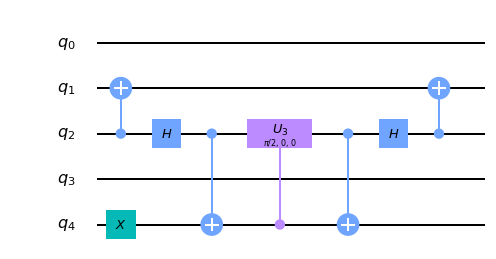
Now, let us consider the circuit implementing the $\sigma_z^{(1)}\otimes\sigma_z^{(2)}$ pump:

To map the eigenspace information into the environment ancilla $a_\textrm{ZZ}$, we apply a CNOT controlled by the relevant qubit, $s_2$. After these two gates (and considering that the initial state of the ancilla is $|1\rangle$), $a_\textrm{ZZ}$ will be in state $|1\rangle$ if the initial state of the system is $| \phi^{\pm} \rangle$ and $|0\rangle$ if it is $| \psi^{\pm} \rangle$. Therefore, the conditional rotation gate only acts in the former case, while it does not modify the state in the latter. The angle of the controlled rotation, in turn, controls the efficiency of the pump $p$ via the relation $\theta = 2 \arcsin{\sqrt{p} }$. Finally, the last two CNOT gates simply revert the mapping part of the circuit.

The working principle of the $\sigma_x^{(1)}\otimes\sigma_x^{(2)}$ pump is essentially the same. However, we need to add an extra Hadamard gate to transform the state of $s_1$ before mapping the information to the ancilla $a_\textrm{XX}$:

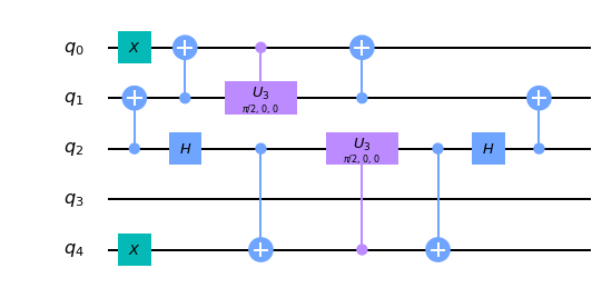
As for the composite pump, we can simply concatenate the two circuits. Notice that in the direct concatenation there would be two consecutive CNOTs between the system qubits, which can be removed.

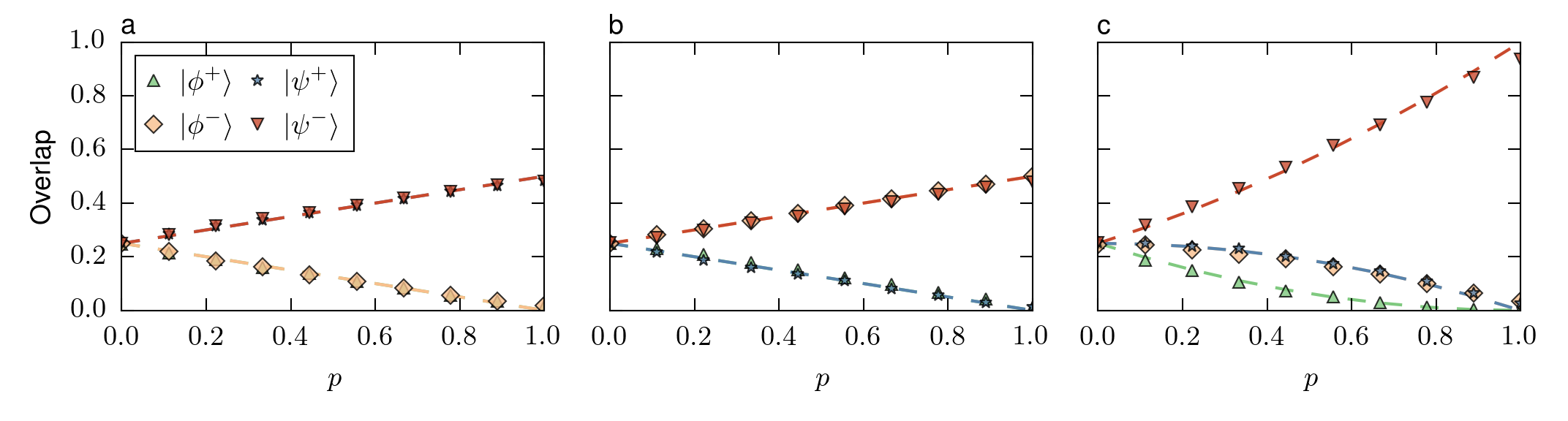
In the figure below we show the action of the dissipative pumping maps $\Phi_{xx}$, $\Phi_{zz}$ and their composition $\Phi_{xx} \circ \Phi_{zz}$ as a function of $p$, for a maximally mixed initial state. We compare the theoretical prediction (dashed lines) with the experimental data. Our results show a very good agreement between theory and experiment for the implementation of both the two families of maps and their composition. In the latter case, the results are more sensitive to errors because of the larger depth of the circuit implementing the composition of maps.

Figure 2. Overlaps with the different Bell states as a function of the efficiency $p$ for the three different channels a) $\Phi_{zz}$, b) $\Phi_{xx}$ and c) $\Phi_{xx} \circ \Phi_{zz}$. The points correspond to the experimental results, while the dashed lines show the theoretical prediction.

Regarding the measurement process, the IBM Q Experience platform only enables measurement in the computational basis. Hence, to assess the probabilities for each of the Bell states, we need to change basis by applying again a combination of CNOT and Hadamard to the system qubits, so $| \phi^{+} \rangle$ is mapped into $|00\rangle$, etc. Again, notice that this would result in repeated consecutive gates, the effect of which amounts to identity, so they can be removed from the circuits. Finally, in Figure 2 we show the results starting from the maximally mixed state. To do so, we simulated the circuits preparing the system in four different initial conditions, $| 00 \rangle$, $| 01 \rangle$, $| 10 \rangle$ and $| 11 \rangle$ and averaged the corresponding results.

References

[1] A. Holevo, Rep. Math. Phys. 32, 211 (1993).

[2] D. Chruściński and S. Maniscalco, Phys. Rev. Lett. 112, 120404 (2014)

[3] J. T. Barreiro, M. Müller, P. Schindler, D. Nigg, T. Monz, M. Chwalla, M. Hennrich, C. F. Roos, P. Zoller, and R. Blatt, Nature 470, 486 (2011)

[4] J. T. Barreiro, P. Schindler, O. Gühne, T. Monz, M. Chwalla, C. F. Roos, M. Hennrich, and R. Blatt, Nat. Phys. 6, 943 (2010).