7.1. The model and its exact solution

We will now study a paradigmatic example of an open quantum system amenable to an exact solution. Solving the dynamics exactly, to all orders in the coupling constant, allows us to compare the exact approach with perturbative TCL solutions.

The physical model we investigate is a two-level atom in a bosonic reservoir at zero temperature. The total Hamiltonian is ($\hbar=1$)

$$ H=H_{S}+H_{E}+H_{I} $$

where

\begin{equation} \begin{aligned} &H_{S}=\frac{\omega_{0}}{2}\sigma_{z},\\ &H_{E}=\sum_{k}\omega_{k}b_{k}^{\dagger}b_{k},\\ &H_{I}=\sum_{k}(g_{k}\sigma_{+}b_{k}+g_{k}^{*}\sigma_{-}b_{k}^{\dagger}), \end{aligned} \label{hams} \tag{7.1} \end{equation}

where $\sigma_{z}$ is the Pauli matrix, $\sigma_{\pm}$ the raising and lowering operators, $b_{k}^{\dagger}, b_{k}$ the bosonic creation/annihilation operators of the environment, the index $\{k\}$ labels the different field modes of the reservoir with frequencies $\omega_k$, and $g_k$ are the coupling constants. The interaction Hamiltonian describes a process where an excitation is exchanged between the system and the environment. It is important to remark that this type of interaction conserves the total number of excitations initially present in the total system, and indeed the existence of this constant of motion is crucial for the derivation of an exact solution. In the following we will derive the exact solution for the total closed system and, from this solution, we will obtain the dynamics of the open system.

Assuming that only one excitation is present in the total system, the total Hilbert space is spanned by the following states $\{|\psi_{0}\rangle=|g\rangle\otimes|0\rangle, |\psi_{1}\rangle=|e\rangle\otimes|0\rangle, |\psi_{k}\rangle=|g\rangle\otimes|1_{k}\rangle\}$, where $|0\rangle=\otimes_{k}|0_{k}\rangle$ is the multimode vacuum state of the reservoir, $|1_{k}\rangle$ denotes the state with one photon in mode $k$ of the environment and $|e\rangle$ and $|g\rangle$ are the excited and ground states of the two-level atom, respectively.

Let us consider the Schrödinger equation in the interaction picture

$$ \frac{d}{dt}|\psi(t)\rangle=-iH_{I}(t)|\psi(t)\rangle $$

where

$$H_{I}(t)=\exp[i(H_{S}+H_{E})t]H_I\exp[-i(H_{S}+H_{E})t]=\sum_{k}g_{k}\sigma_{+}(t)b_{k}(t)+g_{k}^{*}\sigma_{-}(t)b_{k}(t)^{\dagger},$$

with $\sigma_{\pm}(t)=\sigma_{\pm}(0)e^{\pm i\omega_{0}t}$ and $b_{k}(t)=b_{k}e^{-i \omega_k t}$.

Since the total number of excitations $N$, given by

$$ N=\sigma_{+}\sigma_{-}+\sum_{k}b_{k}^{\dagger}b_{k} $$

is a constant of motion, i.e. $[H,N]=0$, the total state of the system $|\psi(t)\rangle$ can be written as

\begin{equation} |\psi(t)\rangle=c_{0}(t)|\psi_{0}\rangle+c_{1}(t)|\psi_{1}\rangle+\sum_{k}c_{k}(t)|\psi_{k}\rangle. \label{psit} \tag{7.2} \end{equation}

Noting that $H_{I}(t)|\psi_{0}\rangle=0$, one can see that the amplitude $c_{0}(t)=c_0$ is constant. Inserting (\ref{psit}) in the Schrödinger equation we get the following set of coupled differential equations for the coefficients

\begin{equation} \begin{cases} \dot{c}_{1}=-i\sum_{k}g_{k}e^{i(\omega_{0}-\omega_{k})t}c_{k}\\ \dot{c}_{k}=-ig_{k}^*e^{-i(\omega_{0}-\omega_{k})t}c_{1}\\ \end{cases} \label{ed1} \tag{7.3} \end{equation}

We can formally solve the equation for the $c_{k}$'s, assuming that $c_k(0) = 0$,

\begin{equation} \begin{aligned} &c_{k}(t)=- ig_{k}^{*}\int_{0}^{t}dt'e^{-i(\omega_{0}-\omega_{k})t'}c_{1}(t') \end{aligned} \label{ed2} \tag{7.4} \end{equation}

and, inserting Eq. (\ref{ed2}) in the equation for $c_1(t)$, we obtain

\begin{equation} \dot{c}_{1}(t)=- \sum_{k}|g_{k}|^{2}\int_{0}^{t}dt'e^{-i(\omega_{0}-\omega_{k})(t-t')}c_{1}(t'). \label{eq:c1} \tag{7.5} \end{equation}

Passing to the continuum limit, i.e. replacing the discrete spectral distribution with a continuous spectral density,

$$ \sum_{k}|g_{k}|^{2}\to\int d\omega J(\omega) $$

we can define the reservoir correlation function $f (t-t')$ as follows

$$ f(t-t')=\int d\omega J(\omega)e^{i(\omega_{0}-\omega)(t-t')}. $$

It is a simple but useful exercise to show that, if the environment is in the vacuum state $\varrho_{B}=|0\rangle \langle0|$, then $\int d\omega J(\omega) e^{-i\omega(t-t')}=\textrm{Tr}_{B}[B(t)B^{\dagger}(t')\varrho_{B}]$, where $B(t)=\sum_k g_k b_k \exp(-i\omega_k t)$. Moreover, if $J(\omega)$ is an integrable function, we can exchange the order of integration in Eq. (\ref{eq:c1}) obtaining

\begin{equation} \dot{c}_{1}(t)=-\int_{0}^{t}dt' f(t-t')c_{1}(t'). \label{integrodiff} \tag{7.6} \end{equation}

The reduced density matrix of the two-level system is obtained from the total system pure state by tracing over the reservoir degrees of freedom:

$$ \begin{aligned} \varrho_{S}(t)&=\textrm{Tr}_{B}\{|\psi(t)\rangle\langle\psi(t)|\}=\langle 0|\psi(t)\rangle\langle\psi(t)|0\rangle+\sum_{k}\langle 1_{k}|\psi(t)\rangle\langle\psi(t)|1_{k}\rangle\\ &=|c_{0}|^{2}|g\rangle\langle g|+c_{0}^{*}c_{1}(t)|g\rangle\langle e|+c_{1}^{*}(t)c_{0}|e\rangle\langle g|\\ &+\sum_{k}|c_{k}(t)|^{2}|g\rangle\langle g|+|c_{1}(t)|^{2}{|e\rangle\langle e|}. \end{aligned} $$

Since $|c_{0}|^{2}+|c_{1}(t)|^{2}+\sum_{k}|c_{k}(t)|^{2}=1$ we can rewrite $\varrho_{S}(t)$ as follows

\begin{equation} \varrho_{S}(t)= \left( \begin{array}{cc} |c_{1}(t)|^{2} & c_{0}^{*}c_{1}(t) \\ c_{0}c_{1}^{*}(t) & 1- |c_{1}(t)|^{2} \end{array} \right). \label{rohs} \tag{7.7} \end{equation}

The equation above shows that the dynamics of the reduced system only depends on the coefficient $c_1(t)$ and on the initial condition $c_0$.

Let us define

\begin{eqnarray} S(t)&=&-2\Im\left[\frac{\dot{c}_{1}(t)}{c_{1}(t)}\right], \label{eq:St} \tag{7.8} \end{eqnarray}\begin{eqnarray} \gamma(t)&=&-2\Re\left[\frac{\dot{c}_{1}(t)}{c_{1}(t)}\right],\label{eq:g} \tag{7.9} \end{eqnarray}

i.e. the time-dependent Lamb shift $S(t)$ and the decay rate $\gamma(t)$ are the imaginary and real part, respectively, of the ratio between the derivative of $c_1(t)$ and the coefficient itself.

By deriving the solution for the reduced density matrix, i.e. Eq. (\ref{rohs}), it is straightforward to show that the master equation is given by

\begin{equation} \frac{d\varrho_{S}}{dt}(t)=-\frac{iS(t)}{2}\left[\sigma_{z},\varrho_{S}(t)\right]+\gamma(t)\left[\sigma_{-}\varrho_{S}(t)\sigma_{+}-\frac{1}{2}\{\sigma_{+}\sigma_{-},\varrho_{S}(t)\}\right]. \label{me} \tag{7.10} \end{equation}

This is the exact master equation for the system dynamics. However, for the equation above to be considered a proper master equation, the Lamb shift $S(t)$ and the decay rate $\gamma(t)$ should be properties of the open system only and should not depend on the initial state of the system. This does not seem to be the case from Eqs. (\ref{eq:St})-(\ref{eq:g}). One should notice that, as Eq. (\ref{integrodiff}) is a first order integro-differential equation, it admits one independent solution only, and in particular it admits a solution of the form $c_1(t) = c f(t)$, with $f(t)$ a time dependent function and $c$ a constant. Hence, the general solution can be written as $c_1(t)=c_1(0) f(t)$, which eliminates the dependence on the initial condition in both $S(t)$ and $\gamma(t)$.

Another important remark is that Eq. (\ref{me}) is exact; however, it is in time local form, i.e. it does not contain memory kernels. One could argue whether this equation always exists (remember our discussion on the existence of the inverse superoperator $(\textrm{I}- \Sigma(t))^{-1}$ in the TCL projection operator derivation). It is easy to see that the time-dependent decay rate diverges if $c_1(t)=0$ (and $\dot{c}_1(t)\neq 0$) for certain time instants. In this case, even if the solution of the master equation is well defined, the master equation is not. In other words a TCL master equation does not exist.

Finally, we note that, in order to apply the method described in this section, we have assumed that the spectral density function is integrable. This is not the case, for example, in certain models of photonic band gap materials, wherein

\begin{eqnarray} J(\omega)= \frac{c}{\sqrt{\omega - \omega_e}} \theta(\omega - \omega_e). \tag{7.11} \end{eqnarray}

7.2. Lorentzian spectral density

A paradigmatic example of an exact model for an open quantum system is the case of a two level atom interacting with the electromagnetic field in the vacuum, with a Lorentzian spectral density

\begin{equation} J(\omega)=\frac{1}{2\pi}\frac{\gamma_{0}\lambda^{2}}{(\omega_{0}-\omega)^{2}+\lambda^{2}}. \label{lor} \tag{7.12} \end{equation}

A Lorentzian spectrum describes, for example the quantized field inside a single mode high Q optical cavity. For this type of spectrum, the correlation function $f(t-t')=\int d\omega J(\omega)e^{i(\omega_{0}-\omega)(t-t')}=\frac{\gamma_{0}\lambda}{2}e^{-\lambda(t-t')}$ describes an exponential decay with rate $\lambda$.

If we now take the Laplace transform of Eq. (\ref{integrodiff}), namely $s\tilde{c}(s)-c(0)=-\tilde{f}(s)\tilde{c}(s)$ (See Appendix 7.4 at the end of this chapter), we get

$$\tilde{c}(s)=\left[\frac{1}{s+\tilde{f}(s)}\right]c(0).$$

Performing the inverse Laplace transform leads to

$$ \begin{aligned} \textrm{Lap}^{-1}\left[\frac{1}{s+\tilde{f}(s)}\right]&=\sum_{k}\frac{1}{(n_{k}-1)!}\left(\frac{d^{(n_{k}-1)}}{ds}\right)\frac{e^{st}}{s+\tilde{f}(s)}(s-p_{k})^{n_{k}}\Bigg |_{s=p_{k}}\\ \\ &= \left(\frac{s_{+}+\lambda}{s_{+}-s_{-}}\right)e^{s_{+}t}+\left(\frac{s_{-}+\lambda}{s_{-}-s_{+}}\right)e^{s_{-}t}. \end{aligned}$$

Hence, we get to the following solution

\begin{equation} c_{1}(t)=c_{1}(0)e^{-\lambda t/2}\left[\cosh\left(\frac{\lambda t}{2}\sqrt{1-2R}\right)+\frac{1}{\sqrt{1-2R}}\sinh\left(\frac{\lambda t}{2}\sqrt{1-2R}\right)\right]. \label{c1lor} \tag{7.13} \end{equation}

where $R=\gamma_{0}/\lambda$. From this equation we can calculate the reduced density matrix elements, e.g. the excited state probability $\varrho_{ee}(t)=\left|c_{1}(t)\right|^{2}$.

Weak and strong coupling

We can switch from weak to strong coupling by varying the $R$ parameter, which quantifies the competitive effects of coupling and dissipation. Figure 1 (left) shows the dynamics of $ρ_{ee}(t)$ in a wide range of values of $R$. The existence of zeros in $ρ_{ee}(t)$ for strong couplings ($R > 1/2$) signals that a TCL master equation does not exist. The right curve depicts the spectral density corresponding to the chosen value of $R$.

Figure 1. This interactive plot shows the dynamics of $ρ_{ee}(t)$ in a wide range of values of $R$ for $\gamma_0 = 1$. The existence of zeros in $ρ_{ee}(t)$ for strong couplings ($R > 1/2$) signals that a TCL master equation does not exist. The right curve depicts the spectral density corresponding to the chosen value of $R$. Drag the slider to change $R$.

Master equation

Recalling Eq.(\ref{eq:g}) we can derive the time dependent decay rate $\gamma(t)$ for the Lorentzian spectrum

$$ \gamma(t)=-2\Re \left\{\frac{\dot{c}_{1}(t)}{c_{1}(t)} \right\} =\frac{2\gamma_{0} \sinh\left(\frac{\lambda t}{2}\sqrt{1-2R}\right)}{\sqrt{1-2R}\cosh\left(\frac{\lambda t}{2}\sqrt{1-2R}\right)+\sinh\left(\frac{\lambda t}{2}\sqrt{1-2R}\right)} $$

which diverges in the strong coupling limit. Formally, this means that the superoperator $[\textrm{I}-\Sigma(t))]^{-1}$ is not defined.

TCL2

Using the TCL projection operator technique one can derive the following time-local master equation

\begin{equation} \frac{d\varrho_{s}(t)}{dt}=\left[\sum_{n=1}^{\infty}\alpha_{n}K_{n}(t)\right]\varrho_{s}(t). \label{tclmast} \tag{7.14} \end{equation}

One can show that the operatorial form of the master equation looks the same at any expansion order (neglecting Lamb-Shift terms)

\begin{equation} \frac{d\varrho_{s}(t)}{dt}=\left[\sum_{n=1}^{\infty}\alpha_{2n}\gamma_{2n}(t)\right]L\varrho_{s}(t) \label{tclmast2} \tag{7.15} \end{equation}

where $L$ is the GKSL operator. To the second order in the coupling constant $\alpha$ we get

$$\gamma_{2}(t)+iS_{2}(t)=2\int_{0}^{t}dt_{1}f(t-t_{1}).$$

For the Lorentzian spectrum we find

\begin{equation} S_{2}(t)=0,\qquad\gamma_{2}(t)=\gamma_{0}(1-e^{-\lambda t}). \label{tcl2} \tag{7.16} \end{equation}

7.3. Markovian and strong coupling limits of the exact solution

Recalling (\ref{c1lor})

$$\varrho_{11}(t)=\Bigg|c_{1}(0)e^{-\lambda t/2}\left[\cosh\left(\frac{\lambda t}{2}\sqrt{1-2R}\right)+\frac{1}{\sqrt{1-2R}}\sinh\left(\frac{\lambda t}{2}\sqrt{1-2R}\right)\right]\Bigg|^{2},$$

where the correlation time of the reservoir is $\tau=1/\lambda$. In the Markovian limit $\lambda\to\infty$ but $\lambda\gamma_{0}$ is constant ($\gamma_{0}\to 0$). In other words the Markovian limit in this model corresponds at taking both a flat reservoir spectrum $\lambda\to\infty$ and very weak coupling $\gamma_{0}\to 0$, the two assumptions are not independent.

By expanding the above equation in the $R\to0$ limit we get

$$ \begin{aligned} c_{1}(t)&\approx c_{1}(0)e^{-\frac{\lambda t}{2}}\left[\frac{e^{(1-2R)\lambda t/2}}{2}+\frac{(1+2R)e^{(1-2R)\lambda t/2}}{2}\right]\\ &= c_{1}(0)e^{-\frac{\lambda t}{2}}e^{(1-2R)\lambda t/2}\approx c_{1}(0)e^{-\frac{R\lambda t}{2}}=c_{1}(0)e^{-\frac{\gamma_{0}t}{2}}. \end{aligned} $$

Hence,

\begin{equation} \varrho_{11}^{\textrm{Mark}}(t)=\varrho_{11}(0)e^{-2\gamma_{0}t}. \label{marklim} \tag{7.17} \end{equation}

This limit also leads to $J(\omega)\to\gamma_{0}/2\pi, f(\tau)\to\gamma_{0}\delta(\tau)$.

In the opposite limit, known as the strong coupling limit, where $\gamma_{0}\to\infty$ and $\lambda\to0$ we have approximately unitary dynamics (Jaynes-Cummings type)

\begin{equation} \varrho_{11}^{\textrm{JC}}(t)\approx\varrho_{11}(0)\cos\left(\frac{\lambda\gamma_{0}}{2}t\right). \label{jclim} \tag{7.18} \end{equation}

Example in Qiskit: Jaynes-Cummings model

To simulate the Jaynes-Cummings model, we consider one qubit as the system ($q_1$) and one extra qubit ($q_2$) to implement the dynamical map. In other words, we do not simulate the dynamics of system and environment, but only the resulting channel on the system qubit. Nevertheless, we will refer to $q_2$ as environment qubit. Given that the only parameter of the channel is $c_1(t)$ (which is itself parametrized by time), the following circuit results in such dynamics:

For an arbitrary pure state of the system $|\psi\rangle_s = \alpha |0\rangle_s + \beta |1\rangle_s$ (notice that we chose $\alpha = 1$ and $\beta = 0$ in the above circuit), and setting the state of the environment to vacuum $|0\rangle_e$, the two gates between the system and environment qubits transform the joint state into $\alpha |0\rangle_s|0\rangle_e + \beta \cos \theta |1\rangle_s|0\rangle_e + \beta \sin \theta |0\rangle_s|1\rangle_e$. Therefore, identifying the states $|0\rangle_s$ and $|1\rangle_s$ with the ground and excited states respectively, and by choosing $\theta = \arccos{c_1(t)}$, the reduced state of the system becomes Eq. (\ref{rohs}).

In Figure 2 we show the experimental results obtained by running this circuit for different values of $t$ on ibmq_vigo.

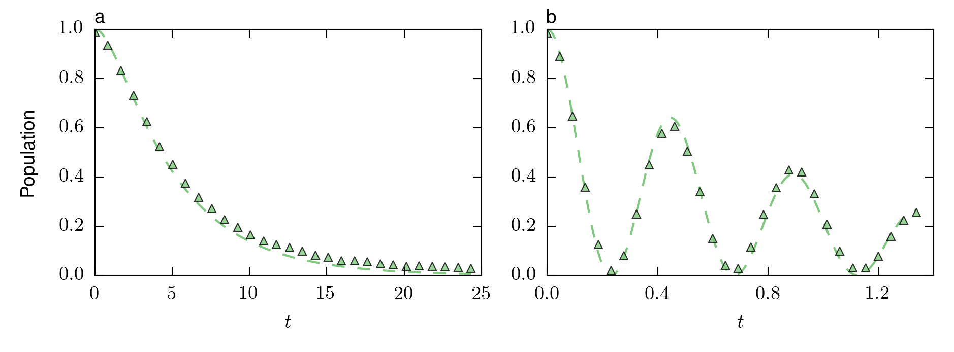
Figure 2. Experimental simulation of the amplitude damping channel. The points show the population of the excited state of the system qubit as a function of the simulation parameter $t$ for different values of the coupling a) $R = 0.2$ and b) $R = 100$. In both cases $\gamma_0 = 1$. The dashed lines show the theoretical prediction.

7.4. Appendix: Some useful properties of Laplace transform

Given a function $f$ we define its Laplace transform $F$ as

$$ F(s)=\textrm{Lap}[f(t)]=\int_{0}^{+\infty}dte^{-st}f(t)=\tilde{f}(s)\qquad s\in\mathbb{C}. $$

Below are some important properties to remember

• $\textrm{Lap}[\alpha f(t)+\beta g(t)]=\alpha\tilde{f}(s)+\beta\tilde{g}(s),$
• $\textrm{Lap}\left[\frac{df}{dt}(t)\right]=s\tilde{f}(s)-f(0),$
• $\textrm{Lap} [f*g(t)]=\tilde{f}(s)\tilde{g}(s),\qquad f*g(t)=\int_{0}^{t}dt_{1}f(t-t_{1})g(t_{1}).$

Also, some important and useful Laplace transforms to keep in mind

• $\textrm{Lap}[\alpha]=\frac{\alpha}{s},$
• $\textrm{Lap}[t]=\frac{1}{s^{2}},$
• $\textrm{Lap}[e^{\alpha t}]=\frac{1}{s-\alpha}\qquad\mathfrak{Re}[s]>\mathfrak{Re}[\alpha].$

The inverse Laplace transform is defined as $$ \textrm{Lap}^{-1}[\tilde{f}(s)]=f(t)=\frac{1}{2\pi i}\int_{\gamma-i\infty}^{\gamma+i\infty}ds e^{st}\tilde{f}(s). $$

In order to compute it we need the Residue theorem $$ \oint_{\gamma}dzf(z)=2\pi i\sum_{k=1}^{n}\textrm{Res}[f,p_{k}], $$

where $\gamma$ is a continuous path in the complex plane and $p_{k}$ is a $n_{k}$ order pole for the function $f$. The residues are defined as

$$ \textrm{Res}[f,p_{k}]=\frac{1}{(n_{k}-1)!}\lim_{z\to p_{k}}\left(\frac{\partial}{\partial z}\right)^{(n_{k}-1)}\left[f(z)(z-p_{k})^{n_{}k}\right]. $$

It immediately follows that $$ \textrm{Lap}^{-1}[\tilde{f}(s)]=\sum_{k=1}^{n}\frac{1}{(n_{k}-1)!}\left(\frac{\partial}{\partial s}\right)^{(n_{k}-1)}\left[e^{st}\tilde{f}(s)(s-p_{k})^{n_{}k}\right]. $$