Non-Markovian quantum dynamics

$\newcommand{\parenthnewln}{\right.\\&\left.\quad\quad{} }$ $\newcommand{\nc}{\newcommand}$ $\nc{\eq}{\begin{equation} }$ $\nc{\eeq}{\end{equation} }$ $\nc{\eqa}{\begin{eqnarray} }$ $\nc{\eeqa}{\end{eqnarray} }$ $\nc{\ar}{\begin{array} }$ $\nc{\ear}{\end{array} }$ $\nc{\bfig}{\begin{figure} }$ $\nc{\efig}{\end{figure} }$ $\nc{\dg}{\dagger}$ $\nc{\eps}{\frac{\epsilon}{2} }$ $\nc{\juuri}{\sqrt{\Omega^2+(\eps)^2} }$ $\nc{\sx}{\sigma_x}$ $\nc{\sy}{\sigma_y}$ $\nc{\sz}{\sigma_z}$ $\nc{\spl}{\sigma_+}$ $\nc{\sm}{\sigma_-}$ $\nc{\Sx}{\bar{\sigma}_x}$ $\nc{\Sy}{\bar{\sigma}_y}$ $\nc{\Sz}{\bar{\sigma}_z}$ $\nc{\Spl}{\bar{\sigma}_+}$ $\nc{\Sm}{\bar{\sigma}_-}$ $\nc{\nn}{\nonumber}$ $\nc{\noi}{\noindent}$ $\nc{\omt}{\tilde{\omega} }$ $\nc{\Somt}{S(\omt)}$ $\nc{\Somtd}{S^{\dg}(\omt)}$ $\nc{\got}{\gamma_{\omega}(t)}$ $\nc{\gmot}{\gamma_{-\omega}(t)}$ $\nc{\po}{\mathcal{P} }$ $\nc{\qo}{\mathcal{Q} }$ $\nc{\adg}{a^{\dg} }$ $\nc{\gammat}{\tilde{\gamma} }$ $\nc{\Q}{\mathcal{Q } }$ $\nc{\C}{\mathcal{C } }$ $\nc{\N}{\mathcal{N} }$ $\nc{\kvec}{\mathbf{k} }$

8.1. Introduction

The last decade has seen a renewed interest in theoretical and experimental investigations on fundamental studies of open quantum systems. The reasons for such interest are manifold. On the one hand, we have witnessed a tremendous advance in the development of quantum technologies, stemming from the ability to coherently control in a robust and efficient manner the dynamics of an ever increasing number of particles. Quantum technologies need to be scalable to reach the market, which entails understanding and minimizing environment-induced decoherence effects in order to achieve the required thresholds for error correction. On the other hand the environment itself has been proven to be experimentally controllable and modifiable. Nowadays reservoir engineering techniques are used for both minimizing the effects of environmental noise and as testbeds of theoretical models.

All recent investigations on open quantum systems dynamics highlight the existence of two different classes of dynamical behavior known as Markovian and non-Markovian regimes. Historically, in the quantum domain Markovian dynamics has been associated to the semigroup property of the dynamical map describing the system evolution. If one thinks in terms of a microscopic model of system, environment and interaction, a Markovian description of the open system requires a number of assumptions, such as system-reservoir weak coupling, and leads to a master equation in the so-called Lindblad form [1, 2]. In certain scenarios, however, such approximations are not justified and one needs to go beyond perturbation theory. It is clear that, due to the general complexity of the problem to be studied, exact solutions exist only for simple open quantum systems models such as the well-known Jaynes-Cummings model [3], the quantum Brownian motion model [4], and certain pure dephasing models [5]-[7].

During the last decade, a new paradigm in the description of open quantum systems has emerged. Specifically, a formal and rigorous information-theoretical approach was introduced and used to define Markovian and non-Markovian dynamics in order to give a clear physical interpretation, as well as an operational definition, to memory effects [8-11, 12]. Markovian dynamics is characterised by a continuous and monotonic loss of information from the open system to the environment while non-Markovian dynamics occurs when part of the information previously lost into the environment comes back due to memory effects, namely information back-flow occurs.

One of the first features that emerges from the analysis of exact models is that memory effects, usually associated to re-coherence and information backflow, do not occur only when the semigroup property of the dynamical map is not satisfied, but are rather associated to another property known as divisibility [13]. In this spirit, a non-Markovianity measure quantifying the deviation from divisibility has been proposed in Ref. [14]. Other measures (and corresponding definitions) are based on the behavior of quantities such as distinguishability between quantum states, as measured, e.g., by trace distance [12, 15] or fidelity [16], quantum mutual information between initial and final state [17], channel capacities [18], Fisher information [19], and the volume of accessible physical states of a system [20].

What one defines as Markovian or non-Markovian dynamics is, in a sense, a question of semantics. It is tautologic to say that, in general, different definitions and corresponding measures of non-Markovianity do not coincide. In this chapter we prefer to follow a more pragmatic approach. We will not insist on the concept of "the best" definition of non-Markovianity but we rather look at different measures as descriptions of different properties of the open quantum systems.

Our study will encompass the Rivas, Huelga, Pleanio (RHP) divisibility measure of [14], the Breuer, Laine, Piilo (BLP) distinguishability measure [12], the Luo, Fu, Song (LFS) coherent information measure [17], and the Bylicka, Chruściński, Maniscalco (BCM) channel capacity measures [18]. We will consider as example single qubits immersed in purely dephasing environments as well as dissipative environments.

8.2. Non-Markovian dynamics: definitions and measures

The concept of Markovian and non-Markovian stochastic process has a clear and rigorous formulation in the classical domain. The extension to quantum processes, however, is not straightforward. Open quantum systems, indeed, may display dynamical features which do not have a classical counterpart, such as re-coherence, information trapping, entanglement sudden death and revivals, and so on. For this reason, the generalization of the definition of Markovian/non-Markovian process from classical to quantum is still the subject of an intense debate (for reviews see Ref. [8-11]). Generally speaking, there are two approaches to the definition of quantum non-Markovianity. The first one focuses on the properties of the master equation or the corresponding dynamical map, while the second one emphasizes the need of a more physical approach, identifying memory effects with the occurrence of information back-flow. The latter approach does not require the knowledge of the explicit form of either the master equation or dynamical map, and has been pioneered by Breuer, Laine and Piilo, who introduced the now famous BLP non-Markovianity measure [12]. In the following we review both perspectives and recall their connection.

8.2.1. Non-Markovianity as non-divisibility

Historically, Markovian open quantum dynamics was identified with the GKSL form of the master equation and was extensively used due to its powerful property of guaranteeing complete positivity (CP), and hence physicality, of the density matrix at all times. A straightforward extension of the GKSL theorem [1, 2] to time local master equations identifies Markovian and non-Markovian dynamics with the properties of the dynamical map $\Phi_t: \rho(t)=\Phi_t \rho(0)$ characterizing the open system evolution. More precisely, the dynamics is said to be Markovian whenever the dynamical map possesses the property of being completely-positive (CP) divisible, namely whenever the propagator $V_{t,s}$, defined by $\Phi_t = V_{t,s} \Phi_s$, is CP. On the contrary, non-Markovian dynamics occurs when the dynamical map $\Phi_t$ is not CP divisible.

A common feature of all non-Markovianity measures described in the following subsections is that they are based on the non-monotonic time evolution of certain quantities occurring when the divisibility property is violated. However, while non-monotonic behavior of such quantities always implies non-divisibility, the inverse is not true, i.e., there can be non-divisible maps consistent with monotonic dynamics. In this sense, if one would assume divisibility as the definition of non-Markovianity, all the other non-Markovianity measures should be considered as non-Markovianity witnesses.

With the defining attribute of all non-Markovian dynamics in mind, namely the violation of the divisibilty property, Rivas, Huelga and Plenio (RHP) propose a measure based on the Choi-Jamiolkowski isomorphism [21]. The inability to write the dynamical map $\Phi_{t}$ as a concatenation of two independent CPTP maps connects with intuitive reasoning of present dynamics being dependent on memory effects.

For master equations written in the standard Lindblad form but with time-dependent coefficients,

\begin{equation} \frac{d \rho_t}{dt}= \mathcal{L}_t \rho_t= -i[H,\rho_t]+ \sum_k\! \! \gamma_k(t) \! \! \left(\! V_k \rho_t V^{\dagger}_k-\frac{1}{2}\{V_k^{\dagger}V_k,\rho_t\}\!\right), \tag{8.1} \end{equation}

it is possible to show that the corresponding dynamical map satisfies divisibility if and only if $\gamma_k(t)\geq0$. If on the other hand, $\gamma_k(t)$ becomes temporarily negative, there will exist an intermediate map $\Phi_{t,t'}$ which is not CPTP, defying the composition law.

According to the Choi-Jamiolkowski isomorphism [21], $\Phi_{t,t'}$ is completely positive if and only if:

\begin{equation} (\Phi_{t,t'}\otimes \mathbb{I})|\Omega \rangle \langle \Omega | \geq 0, \tag{8.2} \end{equation}

where $| \Omega \rangle$ is a maximally entangled state of the open system with an ancilla. In light of this, one can quantify non-Markovianity by considering the departure of the intermediate map from a map which is completely positive [14]:

\begin{equation} \mathcal{N}_{\text{RHP} }=\int_{0}^{\infty} dt\:g(t), \label{RHP_One} \tag{8.3} \end{equation}

where \begin{equation} \label{g} g(t)=\lim_{\epsilon\rightarrow0^+}\frac{||[\mathbb{I}+(\mathcal{L}_t\otimes\mathbb{I})\epsilon]|\Omega \rangle \langle \Omega |\ \ ||_{1}-1}{\epsilon}. \tag{8.4} \end{equation}

and $\epsilon$ encapsulates the time elapsed between the initial time $t'$ to the final time $t$.

Mathematically, an apparent advantage of this measure is that no optimization over states is required. The measure is most simple to calculate using only the specific form of the master equation. However, Eq. (\ref{g}) may be also calculated in terms of the intermediate dynamical map $\Phi_{t,t'}$ [14].

8.2.2. Non-Markovianity as information back-flow

The evolution of a quantum system interacting with its surrounding environment, be it classical or quantum, relativistic or non-relativistic, can be described in terms of exchange of energy and/or information between the two interacting parties. While the concept of energy is uniquely defined in quantum systems, a unique definition of information is lacking. Indeed, in principle, there are a number of useful and rigorous choices for quantifying information, and hence information flow, and such choices obviously depend on which "type" of information one is interested in. Quantum information theory deals with the study of information quantifiers, their properties, their dynamics, and their usefulness in quantum computation, communication, metrology and sensing. In the following we will review different non-Markovianity measures based on different quantifiers of information and, hence, of information flow.

8.2.2.1. Breuer, Laine, Piilo (BLP) Measure

The first attempt to quantify system-environment information flow, and connect it to the Markovian or non-Markovian nature of the dynamics, was based on the concept of trace distance between two states $\rho_1$ and $\rho_2$ of an open system,

\begin{equation} D(\rho_1,\rho_2) = \tfrac{1}{2} \text{tr}\vert \rho_1-\rho_2 \vert . \tag{8.5} \end{equation}

The trace distance is invariant under unitary transformations and contractive for CP dynamical maps, i.e., given two initial open-system states $\rho_1(0)$ and $\rho_2(0)$, the trace distance between the time-evolved states never exceeds its initial value $D[\rho_1(t),\rho_S(t)] \leq D[\rho_1(0),\rho_2(0)]$.

Trace distance is a measure of information content of the open quantum system since it is simply related to the maximum probability $P_D$ to distinguish two quantum states in a single-shot experiment, namely $P_D=\frac{1}{2}[1+D(\rho_1,\rho_2)]$ [22]. Therefore, an increase in trace distance signals an increase in our information about which one of the two possible states the system is in. Following Ref. [12], one can define information flow as the derivative of trace distance as follows:

\begin{equation} \sigma(t)= \frac{d}{dt} D[\rho_1(t),\rho_2(t)]. \tag{8.6} \end{equation}

Even though trace distance cannot increase under CP maps, it may not behave always in a monotonic way as a function of time. Specifically, whenever the trace distance decreases monotonically, information flow is negative, meaning that the system continuously lose information due to the presence of the environment. On the other hand, if for certain time intervals information flow becomes positive, then this signals a partial and temporary increase of distinguishability and, correspondingly, a partial recover of information. This information back-flow has been proposed as the physical manifestation of memory effects and non-Markovianity. This idea is known as BLP non-Markovianity.

Note that, whenever the dynamical map is BLP non-Markovian, i.e., in presence of information back-flow, then it is also CP non-divisible. However, the inverse is not true, namely, there exist systems that are CP non-divisible but BLP Markovian. In general, the concept of non-divisibility and the concept of BLP non-Markovianity, or information back-flow quantified by trace distance, do not coincide and their relationship has been the subject of numerous studies (see, e.g., Ref. [10, 11] for reviews).

Based on this approach, the BLP measure of non-Markovianity $\mathcal{N}_{\text{BLP} }$ is defined by summing over all periods of non-monotonicity of the information flow, including an optimization over all pairs of initial states of the system:

\begin{equation} \mathcal{N}_{\text{BLP} }(\Phi_t)=\max_{\rho^{1,2}_0}\int_{\sigma>0}dt\:\sigma(t). \tag{8.7} \end{equation}

The non-additivity of this measure has been numerically proven, highlighting the challenge presented when one wishes to consider higher dimensional systems of qubits [23]-[25]. Proofs of specific mathematical attributes of the optimal state pairs have to some degree eased the numerical challenges of this calculation by eliminating regions of the $n$-dimensional Hilbert space one should consider [26]. Indeed, it has been shown that the states which maximize the measure must lie on the boundary of the space of physical states and must be orthogonal. Finally, we note that in the spirit of this measure, trace distance is not a unique monotone distance and one may also use others such as the statistical distance [27].

8.2.2.2. Luo, Fu, Song (LFS) Measure

Luo, Fu and Song in Ref. [17] introduced a measure of non-Markovianity based on the monotonicity property characterizing the time-evolution of correlations between system and ancilla when the dynamics are divisible. They focus on the total correlations, including both classical and quantum, captured by the quantum mutual information

\begin{equation} I(\rho_{SA})=S(\rho_S)+S(\rho_A)-S(\rho_{SA}), \tag{8.8} \end{equation}

where $\rho_S=\rm{tr}_A\rho_{SA}$ and $\rho_A =\rm{tr}_S \rho_{SA}$ are marginal states of a system and ancilla, respectively, and $S(\rho)$ is von Neumann entropy of state $\rho$. The LFS approach associates non-Markovianity to a memory-induced restoration of previously lost total (quantum + classical) correlations between an open quantum system and an ancilla, as measured by the mutual quantum information. In this case, therefore, memory effects manifest themselves as a partial and temporary return of mutual information between system and ancilla.

The definition of this measure of non-Markovianiy goes as follows

\begin{equation} \mathcal{N}_{\text{LFS} }(\Phi)=\sup_{\rho^{SA} } \int_{\frac{d}{dt} I >0} \frac{d}{dt} I(\rho_t^{SA}) dt, \label{troppocomplicata} \tag{8.9} \end{equation}

where $\rho^{SA}$ is the initial state of a system plus ancilla and $\rho^{SA}_t=(\Phi_t \otimes \mathbb{I}) \rho_{SA}$. The authors insist that the optimization of the formula above is done over all possible initial states $\rho_{SA}$, where not only the state of the ancilla but also its Hilbert space is arbitrary. Of course this makes the optimization problem extremely complicated. Therefore the authors [17] also propose a simpler version of this measure without optimization

\begin{equation} \mathcal{N}_{\text{LFS}_0}(\Phi)= \int_{\frac{d}{dt} I >0} \frac{d}{dt} I(\rho_t^{SA}) dt, \label{tropposemplice} \tag{8.10} \end{equation}

where $\rho^{SA}_t=(\Phi_t \otimes \mathbb{I}) |\Psi \rangle \langle \Psi|$ and $|\Psi \rangle$ is an arbitrary maximally entangled state.

When the initial state $\rho_{SA}$ is pure, and also the initial state of the environment with which the system is interacting, one can rewrite $I(\rho_{SA})$ as the mutual information between the input and output of the channel defining the system evolution,

\begin{equation} \label{NI} I(\rho, \Phi_t)=S(\rho)+S(\Phi_t \rho )-S(\rho,\Phi_t), \tag{8.11} \end{equation}

with $S(\rho)$ the von Neumann entropy of the input state, $S(\Phi_t \rho)$ the entropy of the output state and $S(\rho,\Phi_t)$ the entropy exchange. Now the non-Markovianity measure reads as

\begin{equation} \mathcal{N}_{\text{I} }(\Phi)=\sup_{\rho} \int_{\frac{d}{dt} I >0} \frac{d}{dt} I(\rho,\Phi_t) dt. \tag{8.12} \end{equation}

The main advantage of $\mathcal{N}_{\text{I} }$ over the original measure $\mathcal{N}_{\text{LFS} }$ is that the optimization has to be done only over the input state of the system.

8.2.2.3. Bylicka, Chruściński, Maniscalco (BCM) Measures

In Ref. [18] two measures that link non-Markovian dynamics with an increase in the efficiency of quantum information processing and communication are introduced. This is motivated by observing that certain capacities of quantum channels are monotonically decreasing functions of time if the channel is divisible. This behavior is a consequence of the connection between the data processing inequality [28] and the divisibility of the dynamical map. In other words, the measures proposed in [18] can be treated as witnesses of non-Markovian dynamics that cause revivals of quantum channel capacities. In other words, these measures physically quantify the total increase, due to reservoir memory, of the maximum rate at which information can be transferred in noisy channels for a fixed time interval or, equivalently, a fixed length of the transmission line.

Let us consider, first, the entanglement-assisted classical capacity $C_{ea}$, which sets a bound on the amount of classical information that can be transmitted along a quantum channel when one allows two parties (Alice and Bob) to share an unlimited amount of entanglement [\ref{NI}), by optimizing over all initial states $\rho$

\begin{equation} C_{ea}(\Phi_t)=\sup_{\rho} I(\rho, \Phi_t). \label{eq:Cea} \tag{8.13} \end{equation}

Since the entanglement-assisted capacity is monotonically decreasing in time when the channel is divisible, any increase of $C_{ea}$ would indicate violation of the divisibility property and so can be considered as a signature of non-Markovianity. Based on this a measure of non-Markovianity was introduced

\begin{equation}\label{NC} \mathcal{N}_{\text{C} }=\int_{ \frac{d C_{ea} }{dt}(\Phi_t) >0} \frac{dC_{ea}(\Phi_t)}{dt} dt, \tag{8.14} \end{equation}

where the integral is extended to all time intervals over which $dC_{ea}/dt$ is positive.

Note that, the calculation of this measure requires optimization only over the input state $\rho$, while the optimization required in the definition of $\mathcal{N}_{\text{BLP} }$ has to be done over pairs of initial states making it much more complicated to calculate, even knowing that we can restrict ourselves to only orthogonal pairs of states (having in mind that beyond the one qubit case more than one corresponding orthogonal state may exist). Thanks to the additivity of the mutual information, one can prove the additivity of $\mathcal{N}_\text{C}$ in the case of $n$ identical independent channels, i.e., $\mathcal{N}_\text{C}(\Phi^{\otimes n})=n \mathcal{N}_\text{C}(\Phi)$.

We now consider a second quantity, namely, the quantum capacity $Q$. This quantity gives the limit to the rate at which quantum information can be reliably sent down a quantum channel and is defined in terms of the coherent information between the input and output of the quantum channel $I_c (\rho, \Phi_t)$ [29]:

\begin{equation} \label{eq:Q} Q(\Phi_t) = \lim_{n \rightarrow \infty} \frac{\max_{\rho_n }I_c(\rho_n,\Phi_t ^{\otimes n})}{n}, \tag{8.15} \end{equation}

with $ I_c(\rho, \Phi_t)=S(\Phi_t \rho)-S(\rho,\Phi_t)$ [30].

Following the same line of reasoning done for $C_{ea}$, a measure of non-Markovianity based on the non-monotonic behavior of the quantum capacity was introduced \begin{equation} \label{NQ} \mathcal{N}_\text{Q}=\int_{\frac{d Q(\Phi_t)}{dt} >0} \frac{d Q(\Phi_t)}{dt} dt, \tag{8.16} \end{equation}

The following interactive plot shows the behaviour of the channel capacity for a qubit undergoing the amplitude damping channel and different values of $R$. It can be seen that, for $R > 40$, the non-Markovianity is already revealed in the chosen time range.

from IPython.display import IFrame

IFrame(src='./gen_plots/channel_cap.html', width=450, height=500)

Figure 1. This interactive plot shows the channel capacity as a function of time for a qubit undergoing the amplitude damping channel dynamics. Drag the slider to see the curve for different values of $R$.

It it worth noting that the two measures of non-Markovianity based on capacities, in general, do not coincide. The distinction between them is actually quite subtle. We notice indeed that as $ I(\rho,\Phi_t) = S(\rho)+I_c(\rho, \Phi_t)$, with $\rho$ the input state, we have $\frac{d}{dt} I(\rho,\Phi_t) = \frac{d}{dt} I_c(\rho, \Phi_t)$. Therefore a measure based on the violation of the data processing inequality for certain non divisible maps and $\mathcal{N}_\text{I}$ would not be able to distinguish between an increase in the different types of correlations. The optimizing state in the definitions (\ref{eq:Cea}) and (\ref{eq:Q}), however, is time dependent and does not coincide for the two quantities, hence $dQ/dt \neq dC_{ea}/dt$.

Contrarily to the entanglement-assisted classical capacity, the quantum channel capacity is in general not additive. However, for degradable channels [31], the general definition coincides with the one-shot capacity, $Q(\Phi_t) = \max_{\rho }I_c(\rho,\Phi_t) $, and additivity for identical independent channels holds.

8.2.3. Connection between non-divisibility and information back-flow

The difference between the concept of CP-divisibility and the concept of memory effects due to information back-flow, as signalled by an increase of distinguishability, can be overcome if one allows for a more general definition of distinguishability between states. More precisely, the concept of distinguishability based on trace distance is based on the idea of equal probabilities of preparing the two states, i.e., the preparation is uniformly random and there is no prior additional information on which one of the two states is prepared. One can, however, generalise this concept by introducing the Helstrom matrix $\Delta$, \begin{equation} \Delta=p_1 \rho_1 - p_2 \rho_2 \tag{8.17} \end{equation}

where $p_1$ and $p_2$ are the prior probabilities of the corresponding states. The information interpretation in terms of the one-shot two-state discrimination problem is valid also in this more general setting [32].

In more detail, one now considers two states and their corresponding ancilla evolving under the CPTP dynamical map $\Phi_t$ as follows

\begin{eqnarray} \rho^{1,2}_{SA}(t)= (\Phi_t\otimes {\cal I}_d) \rho^{1,2}_{SA}(0), \tag{8.18} \end{eqnarray}

with $ \rho_{SA}$ the combined system-ancilla state, ${\cal I}_d$ the identity map, and $d$ the dimension of the Hilbert space of the system, which in this case is equal to the one of the ancilla.

It has been recently shown in Ref. [32] that, for bijective maps, the trace norm of the Helstrom, matrix defined as,

\begin{eqnarray} E(t) = |\Delta(t)|=|p_1 \rho^{1}_{SA}(t) - p_2 \rho^{2}_{SA}(t)| \tag{8.19} \end{eqnarray}

is monotonically decreasing iff the map is CP-divisible. This result has been generalised to non-bijective maps in Ref. [33]. This allows one to interpret lack of CP-divisibility in terms of information back-flow for system and ancilla, when having prior information on the state of the system.

Finally, one can release the assumption of prior information and prove that, if one uses a $d+1$ dimensional ancilla, then the dynamical map $\Phi_t$ is CP-divisible if and only if the trace distance $D$ decreases or remains constant as a function of time for all pairs of initial system-ancilla states Ref.[18]. Therefore, also in this case, one can interpret the loss of CP-divisibility in terms of information back-flow for the system-ancilla pair. For further details on the connection between CP-divisibility and information back-flow we refer the reader to the recent perspective article [11].

8.3. Example: Non-Markovian Pure Dephasing Dynamics

In this section we consider, as a first example, the dynamics of a single qubit interacting with an environment leading to pure dephasing. Note that, as there is no general monotonicity relation between the different non-Markovianity measures, it does not make sense to compare their absolute values. Therefore, in the following we renormalize all measures to take values between zero and 1, and we look at both their qualitative behavior and the Markovian to non-Markovian crossover when certain physical parameters of the model are changed.

A microscopic model of the total system-environment dynamics leading to pure dephasing was derived in Refs. [5]-[7]. One of the advantages of this model is that it is amenable to an exact solution [5]-[7]. We will consider initially the case of a single qubit interacting with a reservoir with spectral density of the Ohmic class. The behavior of all non-Markovianity measures in this case has been studied in Refs. [12], [34]-[36].

The dynamics of a purely dephasing single qubit is captured by the time-local master equation [37]:

\begin{equation} \label{twoqubit} \mathcal{L}_t\rho_t=\gamma_1(t)\left[\sz\rho_t\sz-\frac{1}{2}\{\sz\sz,\rho\}\right], \tag{8.20} \end{equation}

with $\gamma_1(t)$ the time-dependent dephasing rate and $\sz$ the Pauli spin operator. The decay of the off-diagonal elements of the density matrix is described by the decoherence factor $e^{-\Gamma(t)}$, where $\Gamma(t)\geq 0$ and, for a zero-temperature bosonic environment [6],

\begin{eqnarray} \Gamma(t)&=&2\int_{0}^{t} dt' \: \gamma_1(t')\nn\\&=&4\int d\omega \: J(\omega) \frac{1-\cos(\omega \tau)}{\omega^2}, \label{gamma0} \tag{8.21} \end{eqnarray}

with $J(\omega)$ the reservoir spectral density [6, 36].

We consider a reservoir spectral density of the form, \begin{equation} J(\omega)=\frac{\omega^s}{\omega_c^{s-1} } e^{-\omega/\omega_c}, \tag{8.22} \end{equation} where $\omega_c$ is the cutoff frequency and $s$ is the Ohmicity parameter.

In this model re-coherence occurs when $\Gamma(t)$ temporarily decreases for certain time intervals, corresponding to a negative value of the dephasing rate $\gamma_1(t)$. One may analytically determine the times $t\in[a_i,b_i]$ encapsulating non-monotonic intervals of $\Gamma(t)$, i.e. corresponding to $\gamma_1(t)=0$, with $i=1, 2, 3,...$ the number of such time intervals. The extremes of the time intervals, $a_i$ and $b_i$, will depend on the Ohmicity parameter $s$, as changing $s$ one changes the form of the reservoir spectral density. In Ref. [38] it is shown that, for $s<2$, $\gamma_1(t) > 0$ at all times, or equivalently $\Gamma(t)$ increases monotonically. For $s\in [2,4]: a_1=\tan\pi/s, b_1=\infty$ and for $s\in [4,6]: a_1=\tan\pi/s, b_1=\tan2\pi/s$, i.e., we only have one time interval of non-monotonic behavior. For $s>6$, $i>1$, i.e., there are more than one interval of time for which the dephasing rates become negative.

We give here the analytical expressions of $\Gamma(t)$ at times $a_i$ and $b_i$ as these will be used in the following.

\begin{eqnarray} \Gamma(a_1)&=\frac{2\tilde\Gamma[s][1+\cos^{s}(\pi/s)]}{s-1} \label{1gamma1} \tag{8.23} \end{eqnarray}\begin{eqnarray} \Gamma(b_1 )&=\frac{2\tilde\Gamma[s][1-\cos^{s}(2\pi/s)]}{s-1} \hspace{0.7 cm} s\in [4,6] \tag{8.24} \end{eqnarray}\begin{eqnarray} \Gamma(b_1)&=2\tilde\Gamma[s-1] \hspace{2.6 cm} s\in [2,4], \label{1gammb1} \tag{8.25} \end{eqnarray}

where $\tilde\Gamma[x]$ is the Euler gamma function

RHP Measure

Inserting Eq. (\ref{twoqubit}) into Eq. (\ref{g}) and using Eq. (\ref{RHPOne}) one immediately obtains the analytical expression for the RHP non-Markovianity measure $\mathcal{N}{\text{RHP} }$ for a single qubit [14]: \begin{equation} \mathcal{N}_{\text{RHP} }=-2\int_{\gamma_1(t)<0}dt\:\gamma_1(t)=\sum_i\Gamma(a_i)-\Gamma(b_i). \label{RHPdephasing} \tag{8.26} \end{equation}

For the sake of simplicity we look at values of the Ohmicity parameter in the interval $0 \le s \le 6$. In this case there is only one interval of negativity of the decay rates and the only values needed are $\Gamma(a_1)$ and $\Gamma(b_{1})$, defined in Eqs. (\ref{1gamma1})-(\ref{1gammb1}).

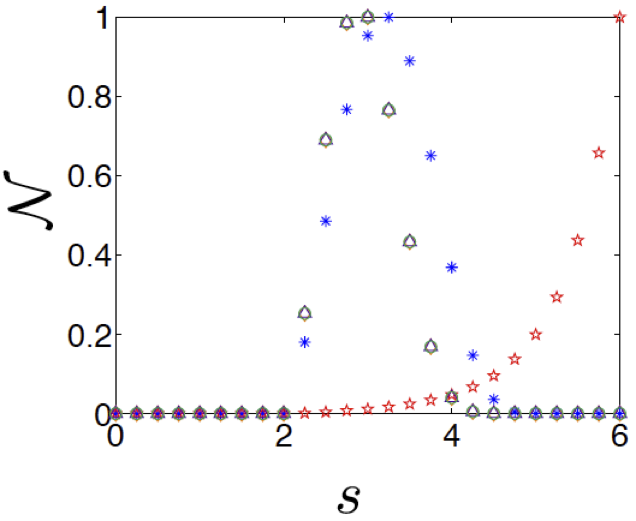
Figure 2. Non-Markovianity measures for a single purely dephasing qubit as a function of the Ohmicity parameter $s$. We show the RHP Measure (red star), the BLP (blue asterisk), the LFS measure (green circle), the quantum capacity measure (purple triangle) and the entanglement-assisted capacity measure (orange diamond). Note that the last three measures in this case coincide. All the measures in this case are normalized to unity. Note that the value of all measures for $s \ge 2$ is always non-zero, even if all measures except RHP take very small values for $s>4$

In Figure 2 we plot $\mathcal{N}_{\text{RHP} }$ for different values of the Ohmicity parameter $s$ (red stars). As one can see from the analytical expression, for increasing $s$ the area of the region of negativity of the dephasing rates increases, hence the measure monotonically increases for higher and higher values of $s$.

BLP Measure

It is straightforward to show that $\mathcal{N}_{\text{BLP} }$ can be written in terms of the two independent elements of the single qubit density matrix [39]

\begin{equation} \mathcal{N}_{\text{BLP} }=-2 \max_{m,n} \int_{\gamma_1<0}\gamma_1(t)\frac{|n|^2e^{-2\Gamma(t)} }{\sqrt{m^2+|n|^2e^{-2\Gamma(t)} }}, \label{BLPone} \tag{8.27} \end{equation}

where $m=\rho_{11}^1(0)-\rho_{11}^2(0)$ and $n=\rho_{12}^1(0)-\rho_{12}^2(0)$, with $\rho^i_{jj} (0)$ the diagonal elements of the initial density matrices of the pair and $\rho_{jk}^i(0)$ their off diagonal elements, with $(i,j,k=1,2)$. This expression shows immediately that $\sigma(t)>0$ iff $\gamma_1(t)<0$; i.e. $\mathcal{N}_{\text{BLP} }\neq 0$ only when the dynamical map is non-divisible [12].

For the model here considered it is possible to analytically solve the optimization problem of Eq. (\ref{BLPone}) [40]. The pair of states optimizing the increase of the trace distance are antipodal states lying on the equatorial plane, e.g., the states $| \pm \rangle=\frac{1}{\sqrt{2} }(| 0 \rangle \pm | 1\rangle)$, with $ | 0 \rangle$ and $| 1 \rangle$ the two states forming the qubit. Hence, we now have: \begin{equation} \mathcal{N}_{\text{BLP} }=\sum_i e^{-\Gamma(b_i)}-e^{-\Gamma(a_i)} \label{NBLPdephasing} \tag{8.28} \end{equation} where again $t\in[a_i,b_i]$ indicates the time intervals when $\gamma_1(t)<0$.

Figure 2 shows the behavior of $\mathcal{N}_{\text{BLP} }$ when changing $s$ (blue asterix). The measure remains non-zero for increasing values of $s$ but, contrarily to the RHP measure it starts decreasing taking small but finite values for $s>3.2$.

LFS Measure

Numerical results show that the optimizing state for this measure is the maximally mixed state [18]. Since $I\left(\frac{\mathbb{I} }{2}, \Phi_t \right)= 2-H_2 \left( \frac{1}{2}+ \frac{e^{-\Gamma(t)} }{2}\right)$, where $H_2(.)$ stands for the binary Shannon entropy, one has

\begin{equation} \frac{d}{dt} I\left(\frac{\mathbb{I} }{2}, \Phi_t \right)=-\frac{1}{2} \gamma_1(t) e^{-\Gamma(t)} \log_2 \left(\frac{1+ e^{-\Gamma(t)} }{1- e^{-\Gamma(t)} }\right), \tag{8.29} \end{equation}

which indicates that the measure $\mathcal{N}_{\text{I} }$ has non-zero value if and only if $\gamma_1(t)<0$, i.e., whenever the dynamical map is non-divisible.

The explicit expression for the measure $\mathcal{N}_{\text{I} }$ is then easily written as

\begin{equation}\label{NID} \mathcal{N}_\text{I}(\Phi_t )=\sum_{i} \left[H_2 \left( \frac{1}{2}+ \frac{e^{-\Gamma(a_i)} }{2}\right)-H_2 \left( \frac{1}{2}+ \frac{e^{-\Gamma(b_i)} }{2}\right) \right]. \tag{8.30} \end{equation}

It is worth noting that in the case of the dephasing channel here considered, for the simple measure without optimization we have, $\mathcal{N}_\text{I}(\Phi_t)=\mathcal{N}_{\text{LFS}_0}(\Phi_t)$.

In Figure 2 we plot $\mathcal{N}_{\text{LFS} }$ as a function of $s$ (green circles). We note that the behavior of this measure is qualitatively similar to that of $\mathcal{N}_{\text{BLP} }$.

BCM Measures

In case of pure-dephasing channels the state optimizing the formula for the classical entanglement assisted capacity is a maximally mixed state, independently of time or of the specific properties of the environmental spectrum. This means that there is a simple analytical formula characterizing it, namely $C_{ea}^D=I(\frac{\mathbb{I} }{2}, \Phi_t)$ [41]. Hence the measures based on mutual information and classical entanglement assisted capacity, in this particular case, coincide: $\mathcal{N}_{\text{C} }(\Phi_t)=\mathcal N_\text{I}(\Phi_t)$.

The dephasing channel is degradable for all admissible dephasing rates $\gamma(t)$, i.e. whenever $\Gamma(t) \ge 0$. This simplifies the calculations of the quantum capacity. Indeed, we find that the state optimizing the coherent information in the definition of the quantum capacity is once again the maximally mixed state. Having this in mind one can show a very simple relation between the two capacities, namely $C_{ea}^D(t) = 1+ Q^D(t)$. It follows immediately that $\mathcal{N}_\text{Q}(\Phi_t)=\mathcal{N}_\text{C}(\Phi_t)=\mathcal N_I(\Phi_t)$.

We conclude this subsection stressing that, for the single qubit case, all non-Markovianity measures detect non-divisibility, hence when studying their behavior as a function of the parameter $s$ we obtain the same crossover between Markovian and non-Markovian dynamics, i.e., $s=2$. A direct comparison between the analytic expressions of Eqs. (\ref{RHPdephasing}), (\ref{NBLPdephasing}) and (\ref{NID}) clarifies the different qualitative behaviour shown by the RHP measure with respect to the other ones in Figure 2. Indeed, the increasing value of the former measure is due to the fact that, for increasing $s$, the number of periods of negativity of the dephasing rate increases and with it the terms contributing to the sum of Eq. (\ref{RHPdephasing}). On the contrary, the other measures all depend on the dephasing factors $e^{-\Gamma(t)}$ calculated at times at which the direction of information flow changes, i.e. $t=a_i$ and $t=b_i$. For increasing values of $s$, in the $s \gtrsim 3$ parameter space, however, $e^{-\Gamma(a_i)} \simeq e^{-\Gamma(b_i)}$, hence the values of both $\mathcal{N}_\text{BLP}$ and $\mathcal{N}_\text{I}(\Phi_t)=\mathcal{N}_\text{Q}(\Phi_t)=\mathcal{N}_\text{C}(\Phi_t)$ decreases, as one can easily see from Eqs. (\ref{NBLPdephasing}) and (\ref{NID}).

8.4. Example: Non-Markovian Amplitude Damping Channel

Let us now consider the case in which the interaction between the quantum system and its environment leads to energy exchange between the two, resulting in dissipative open system dynamics. We will focus on exemplary open system models amenable to an exact analytical solution as this allows us to gain a solid understanding of the physical phenomena associated with reservoir memory. We consider a single qubit interacting with a quantized bosonic field with both Lorentzian and Photonic Band Gap (PBG) spectra.

8.4.1. The model

The dynamics of a single amplitude damped qubit is captured by the time-local master equation [37]:

\begin{equation} \frac{d\rho_t}{dt}=\gamma_1(t)\left[\sigma_{-}\rho\sigma_{+}-\frac{1}{2}\{\sigma_{+}\sigma_{-},\rho_t\}\right], \label{master} \tag{8.31} \end{equation}

where $\sigma_{\pm}$ are the spin lowering and rising operators and

\begin{equation} \gamma_1(t)=-2\Re\frac{\dot{G}(t)}{G(t)}. \label{gammaADC} \tag{8.32} \end{equation}

The function $G(t)$ depends on the form of the reservoir spectral density.

If the spectral density has a Lorentzian shape, i.e, $J(\omega)=\gamma_M\lambda^2/2\pi[(\omega-\omega^2)+\lambda^2]$, then the function $G^L(t)$ takes the form:

\begin{equation} G^L(t)=e^{-\frac{(\lambda-i\delta)t}{2} }\left[\text{cosh}\left(\frac{\Omega t}{2}\right)+\frac{\lambda-i\delta}{\Omega}\text {sinh}\left(\frac{\Omega t}{2}\right)\right], \tag{8.33} \end{equation}

with \begin{equation} \omega=\sqrt{\lambda^2-2i\delta \lambda -4\omega^2} \tag{8.34} \end{equation} where $\omega=\gamma_M\lambda/2+\delta^2/4$ and $\delta=\omega_0-\omega_c$.

For $\delta=0$, one obtains the following solution

\begin{eqnarray} G^L(t)&=&e^{-\lambda t/2}\left[\text{cosh}\left(\sqrt{1-2r}\frac{\lambda t}{2}\right)\right.\nn\\&+&\left.\frac{1}{\sqrt{1-2r} }\text{sinh}\left(\sqrt{1-2r}\frac{\lambda t}{2}\right)\right] \tag{8.35} \end{eqnarray}

with $r=\lambda_M/\lambda$.

For the Photonic Band Gap model, the specific form of $G^P(t)$ is as follows [42]:

\begin{eqnarray} G^P(t)&=&2v_1x_1e^{\beta x_1^2+i\Delta t}+v_2(x_2+y_2)e^{\beta x_2^2 t+i \Delta t}\nn\\&-&\sum_{j=1}^{3}a_jy_j[1-\Phi(\sqrt{\beta x^2_j t})e^{\beta x^2_j t+i\Delta t}]. \tag{8.36} \end{eqnarray}

where $\Delta=\tilde\omega_0-\omega_e$ is the detuning from the band gap edge frequency $\omega_e$, set to equal zero as we consider only the resonant case. In addition:

\begin{eqnarray} & & x_1=(A_++A_-)e^{i(\pi/4)},\nn\\& & x_2=(A_+e^{-i(\pi/6)}-A_-e^{i(\pi/6)})e^{-i(\pi/4),} \nn\\& & x_3=(A_+e^{i(\pi/6)}-A_-e^{-i(\pi/6)})e^{i(3\pi/4)}, \tag{8.37} \end{eqnarray}\begin{equation} A\pm=\left[\frac{1}{2}\pm\frac{1}{2}\left[1+\frac{4}{27}\frac{\Delta^3}{\beta^3}\right]^{1/2}\right]^{1/3}, \tag{8.38} \end{equation}\begin{equation} v_j=\frac{x_j}{(x_j-x_i)(x_j-x_k)} \: \:(j\neq i\neq k;j,i,k=1,2,3), \tag{8.39} \end{equation}\begin{equation} y_j=\sqrt{ {x_j}^2} \: (j=1,2,3), \tag{8.40} \end{equation}\begin{equation} \beta^{3/2}=\omega_0^{7/2}d^2/6\pi\epsilon_0\hbar c^3. \tag{8.41} \end{equation}

The coefficient $\beta$ is defined as the characteristic frequency, $\epsilon_0$ the Coulomb constant and $d$ the atomic dipole moment. We have defined in our results $z=\Delta/\beta$.

In general, for the exact amplitude damping channel, the state of the density matrix of the qubit at time $t$ can be written in terms of the initial density matrix elements $\rho_{ij}$ ($i,j=1,2$) as follows

\begin{equation} \rho_t = \begin{pmatrix} 1-|G(t)|^2\rho_{22}&G(t)\rho_{12}\\ \\ G^*(t)\rho_{12}^*&|G(t)|^2\rho_{22}\\ \end{pmatrix}. \tag{8.42} \end{equation}

8.4.2. The Non-Markovianity measures

RHP Measure

Since the master equation is in GKSL form with time-dependent coefficients it is straightforward to evaluate the RHP measure for a generic spectral density [39]. \begin{equation} \mathcal{N}_{\text{RHP} }=-\int_{\gamma_1(t)<0}dt\:\gamma_1(t). \tag{8.43} \end{equation}

We consider first the case of a Lorentzian spectrum \begin{equation} J(\omega)=\frac{\gamma_M\lambda^2}{2\pi[(\omega-\omega_c)^2+\lambda^2]}, \tag{8.44} \end{equation}

with $\gamma_M$ an effective coupling constant, $\lambda$ the width of the Lorentzian and $\omega_c$ the peak frequency. When the qubit frequency $\omega_0$ coincides with $\omega_c$ (resonant Jaynes-Cummings model), the dynamical map is non-divisible for $r>r_{\text{crit} }=0.5$, with $r=\gamma_M/\lambda$ [37]. From this critical value $\mathcal{N}_{\text{RHP} }$ diverges as a direct consequence of the divergent behavior of $\gamma_1(t)$. Conversely, in the weak coupling regime, i.e. $r<0.5$, $\gamma_1(t)$ is positive for all times and hence the channel is always divisible ($\mathcal{N}_{\text{RHP} }=0$).

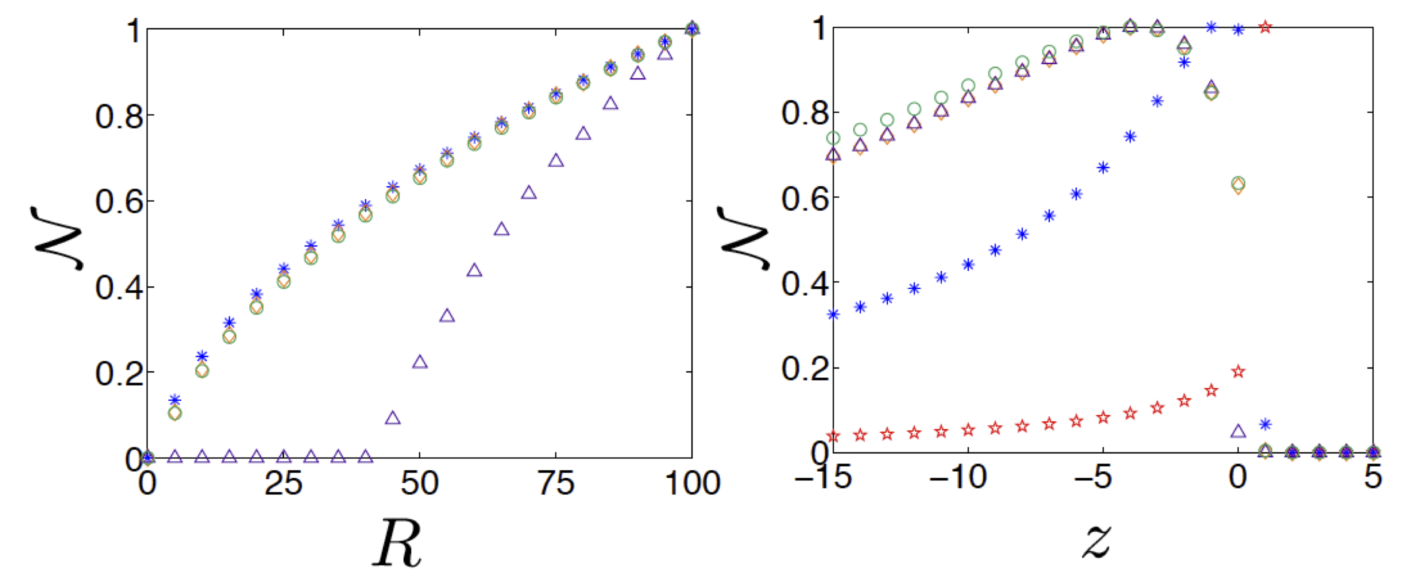
Figure 3. Non-Markovianity measures for a qubit undergoing amplitude damping for i) Lorentzian spectrum (left figure) and ii) Photonic Band Gap model (right figure). We plot the RHP measure (red star), the BLP measure (blue asterisk), the LFS measure (green circle), the quantum capacity measure (purple triangle) and the entanglement-assisted capacity measure (orange diamond). All the measures in this case are normalized to unity. We consider the following times periods: i) $0 \le \lambda t \le 40$ and ii) $0 \le \beta t \le 20$. For the Lorentzian spectrum, the RHP measure is zero for $r \le 0.5$ while it diverges for $r>0.5$.

For the PBG model [\ref{gammaADC}) and (8.55) we can study the Markovian to non-Markovian crossover as a function of the reservoir parameter $z=\Delta/\beta$, with $\Delta$ the detuning of the qubit frequency from the edge frequency $\omega_e$ of the band gap spectrum, and $\beta$ a characteristic frequency. Positive values of $z$ correspond to the case in which the qubit is outside the band gap region while negative values of $z$ correspond to the qubit in the band gap region. In the latter case the well-known phenomenon of population trapping occurs as the emission of energy in the reservoir is strongly inhibited.

For $z<z_{\text{crit} }=1.7$, the rate $\gamma_1 (t)$ temporarily attains negative values for certain time intervals. In fact, due to population trapping, for $z \ll z_{\text{crit} }$ the asymptotic long time limit is characterized by small amplitude oscillations between positive and negative values which persist as $t \rightarrow \infty$. This eventually leads to a divergency not only of the $\mathcal{N}_{\text{RHP} }$ measure but of all non-Markovianity measures. In any practical experimental situation, however, the time of the experiment is finite. We will therefore calculate the measures for a fixed time interval, longer compared to the typical times of the system but, of course, shorter than the system-reservoir correlation time which in this case is $\infty$.

In Figure 3 ii) we plot the RHP measure (red stars) for the PBG reservoir as a function of the parameter $z$. As we can see from the plot the measure has a sudden peak at values of $z$ close to the edge $z=0$, reaching its maximum value for $z=1.0$ before vanishing for $z=1.7$. For increasingly negative values of $z$ under the critical point, RHP non-Markovianity measure decreases to small but finite values. This is due to the decreasing amplitude of the oscillations in the decay rate.

BLP Measure

We begin by deriving the analytical expression for $\mathcal{N}_{\text{BLP} }$ [39]:

\begin{equation} \mathcal{N}_{\text{BLP} }=- \max_{m,n} \int_{\gamma_1<0}\gamma_1(t)\frac{|G(t)|^3m^2+0.5|G(t)||n|^2}{\sqrt{|G(t)|^2m^2+|n|^2} }. \tag{8.45} \end{equation}

where $m=\rho_{11}^1(0)-\rho_{11}^2(0)$ and $n=\rho_{12}^1(0)-\rho_{12}^2(0)$ are coefficients to be optimized. We have compelling numerical evidence that the maximizing states are the orthogonal states $| + \rangle \langle + |$ and $|- \rangle \langle -|$ for both the Lorentzian and the PBG spectral densities for any time $t$. Hence the BLP measure takes the form

\begin{equation} \mathcal{N}_{\text{BLP} }=-\frac{1}{2}\int_{\gamma_1<0}\gamma_1(t)|G(t)|. \label{NBLPADC} \tag{8.46} \end{equation}

As we expect when only one decay rate is present in the master equation, $\mathcal{N}_{\text{BLP} }\neq 0$ if and only if the dynamics are non-divisible i.e., $\gamma_1(t)<0$.

Figure 3 shows $\mathcal{N}_{\text{BLP} }$ (blue asterisk) for different values of i) $r$ and ii) $z$ for the Lorentzian and PBG spectra, respectively. The behavior is qualitatively similar to the one of the RHP measure. In the PBG case the peak of non-Markovianity is slightly shifted towards more negative values of $z$. In Ref. [43], the BLP measure and RHP witness are calculated for quantum harmonic oscillators in a band gap showing that both measures are sensitive to the edge of the gap, which is what we also observe.

BCM and LFS Measures

For the amplitude damping channel the quantum and entanglement-assisted classical capacities, which we indicate here with $Q^A$ and $C_{ea}^A$, respectively, are calculated numerically [44, 45]. The states optimizing $I_c(\rho_t, \Phi_t)$ and $I(\rho_t, \Phi_t)$ are now time-dependent. One finds [46] the following formulas $C_{ea}^A = \max_{p\in [0,1]} \Big\{ H_2(p) + H_2(|G(t)|^2p) - H_2([1-|G(t)|^2]p)\Big\}$, and $Q^A = \max_{p\in [0,1]} \Big\{ H_2(|G(t)|^2p) - H_2([1-|G(t)|^2]p)\Big\}$, which still need a simple optimization over the probability $p\in [0,1]$. The latter formula holds only for $|G(t)|^2 > \frac 12$, otherwise $Q(\Phi^A_t)\equiv 0$. This is due to the fact that the amplitude damping channel is degradable for $|G(t)|^2>\frac{1}{2}$, while for $|G(t)|^2 \le \frac{1}{2}$ is anti-degradable with zero quantum capacity.

The behaviour of the BCM and LFS measures in the two cases of amplitude damping channels is illustrated in Figure 3. For both the Lorentzian reservoir spectrum and the PBG the measures $\N_{\text{C} }$ and $\N_\text{I}$ take non-zero values if and only if the amplitude damping channel is non-divisible. Notice that the measures $\N_\text{I}$ and $\N_\text{C}$ have very close values. This may seem not surprising given that both measures are based on quantum mutual information. However, the examples show that there is no relation between them even in the simple amplitude damping model here considered. Indeed a strong dependence on the form of the environmental spectrum can be noticed. More precisely, in the case of the Lorentzian spectrum we have $\N_\text{C}(\Phi^A)>\N_\text{I}(\Phi^A)$, while in the PBG model the opposite relation holds (see Figure 3 i) and ii), respectively).

We would like to emphasize the difference in the behavior of $\N_\text{Q}$ for the Lorentzian reservoir spectrum. As shown in Figure 3 i), indeed, unlike the other measures $\N_\text{Q}$ is equal to zero even for a non-divisible channel and detects non-Markovianity only in a very strong coupling regime, i.e. when $r>43$. The above example is consistent with the intuitive idea that the transmission of quantum information along a quantum channel is more sensitive to noise than the transmission of classical information (although assisted by entanglement shared between Alice and Bob). Once again this conclusion is, however, spectrum-dependent. In the case of the PBG model (Figure 3 ii)) it is possible to set the parameters such that the noise in the channel has almost the same effect on both kinds of information. This is possible for $z<0$, because $|G(t)|^2$ in this regime oscillates only above the value $\frac{1}{2}$, but it is no longer true for $0\leq z < 2$ as shown in Figure 3 ii) -- the biggest difference occurring for $z=0$.

IBM Q example: Amplitude damping channel

In previous chapter we obtained an exact solution for Jaynes-Cummings model with losses, which is a generalised amplitude damping model. The master equation is given by Eq. (7.10), where the time dependent decay rate $\gamma(t)$ has the following analytical form

\begin{equation} \label{ampD} \gamma(t)=-2\Re\left[\frac{\dot{c}_{1}(t)}{c_{1}(t)}\right], \end{equation}

with \begin{eqnarray} c_{1}(t)&=&c_{1}(0)e^{-\lambda t/2}\left[\cosh\left(\frac{\lambda t}{2}\sqrt{1-2R}\right) + \frac{1}{\sqrt{1-2R} }\sinh\left(\frac{\lambda t}{2}\sqrt{1-2R}\right)\right]. \label{c1lor} \end{eqnarray}

It is a straightforward calculation to show that the time-dependent decay rate $\gamma(t)$ takes negative values for certain time intervals whenever $2 R\ge 1$. In this case the dynamical map is not CP-divisible, and therefore non-Markovian. The left plot in interactive Figure 4 below shows the population of the excited state. It can be seen that, for small $R$, it decays monotonically, while the population oscillates for large values of $R$, since the qubit exchanges information and energy with the central mode of the Lorentzian peak, resonant with the qubit's Bohr frequency.

We also implement an experimentally friendly witness of non-Markovianity proposed in Ref. [47] which stems from the spectral properties of the dynamical map. The witness is based on the behaviour of an initial maximally entangled state of qubit and auxiliary ancilla, and requires only the measurement of the expectation values of local observables such as $\sigma_i \otimes \sigma_i$, ($i=x,y,z$). Non-monotonic behaviour of the witness as a function of time signals non-Markovianity. Other witnesses of non-Markovianity (such as the BLP measure [12]) could be implemented, and may be more efficient at detecting memory effects, but they generally require a larger number of measurements or optimization over initial states.

from IPython.display import IFrame

IFrame(src='./gen_plots/nonmark_witness.html', width=700, height=350)

Figure 4. The left plot shows the population of the excited state of a qubit undergoing the amplitude damping channel dynamics, while the right plot depicts the value of the non-Markovianity witness. Drag the slider to modify the value of $R$.

Here we will use as a basis the circuit from previous chapter and add to it the non-Markovianity witness. The non-Markovianity witness for the mentioned above channel proposed in Ref. [47] is based on the dynamical behaviour of the entanglement between the system and an ancilla initially prepared in a maximally entangled state. Namely, this quantity is defined as $f_{\Phi} = \langle \phi^{+} | \mathbb{I} \otimes \Phi_t [| \phi^{+} \rangle \langle \phi^{+} | ] | \phi^{+} \rangle$. Hence, implementing this quantity requires preparing the state $| \phi^{+} \rangle$ between the system and an ancilla, which can be achieved using a Hadamard and a CNOT gates, applying the dynamical map to the system and measuring the probability of finding the joint system and ancilla state in $| \phi^{+} \rangle$. Figure 4 (right plot) also depicts the behaviour of the witness for different values of $R$, and shows its oscillations in the non-Markovian regime. As suggested in Ref. [47], we need not use an extra CNOT gate to project on the Bell basis; instead, we can take advantage of the fact that $| \phi^{+} \rangle \langle \phi^{+} | = (\mathbb{I}\otimes \mathbb{I} + \sigma_{x}\otimes \sigma_{x} - \sigma_{y}\otimes \sigma_{y} + \sigma_{z}\otimes \sigma_{z})/4$ and measure the corresponding local observables. We now show the circuit corresponding to the measurement of $\sigma_{y}\otimes \sigma_{y}$.

#######################################
#  Amplitude damping channel          #
#   with non-M. witness on IBMQ_VIGO  #
#######################################
from qiskit import QuantumRegister, ClassicalRegister, QuantumCircuit
# Quantum and classical register
q = QuantumRegister(5, name='q')
c = ClassicalRegister(2, name='c')

# Quantum circuit
ad = QuantumCircuit(q, c)

# Amplitude damping channel acting on system qubit
# with non-Markovianity witness
## Qubit identification
system = 1
environment = 2
ancilla = 3

# Define rotation angle
theta = 0.0

# Construct circuit
## Bell state between system and ancilla
ad.h(q[system])
ad.cx(q[system], q[ancilla])

## Channel acting on system qubit
ad.cu3(theta, 0.0, 0.0, q[system], q[environment])
ad.cx(q[environment], q[system])

## Local measurement for the witness
### Choose observable
observable = 'YY'
### Change to the corresponding basis
if observable == 'XX':
    ad.h(q[system])
    ad.h(q[ancilla])
elif observable == 'YY':
    ad.sdg(q[system])
    ad.h(q[system])
    ad.sdg(q[ancilla])
    ad.h(q[ancilla])
### Measure
ad.measure(q[system], c[0])
ad.measure(q[ancilla], c[1])

# Draw circuit
ad.draw(output='mpl')

In Figure 5, we plot the experimental results of the entanglement witness for the amplitude damping channel. The witness clearly shows oscillatory behaviour, and therefore properly signals the presence of memory effects.

Figure 5. Dynamical behaviour of the non-Markovianity witness for a) $R=0.2$ and b) $R=100$. The dots correspond to the experimental results simulated on ibmq_vigo, while the dashed curves show the theoretical prediction.

8.5. Appendix: Mathematical Description of Physical Models

In this Appendix, we present in detail the mathematical description of each system considered in this work.

8.5.1. Purely Dephasing Model

One Qubit

The Hamiltonian of the system is given as [6]:

\begin{equation} H=\omega_0\sigma_z+\sum_k\omega_k a^{\dagger}_ka_k+\sum_k\sigma_z(g_za_k+g^*_ka_k^{\dagger}), \tag{8.47} \end{equation}

with $\omega_0$ the qubit frequency, $\omega_k$ the frequencies of the reservoir modes, $a_k(a_k^{\dagger})$ the annihilation (creation) operators of the bosonic environment and $g_k$ the coupling constant between each reservoir mode and the qubit. In the continuum limit $\sum_k|g_k|^2\rightarrow\int d\omega \: J(\omega) \delta (\omega_k-\omega)$, where $J(\omega)$ is the reservoir spectral density [6, 36].

It is simple to obtain the operator-sum representation $\phi^D_t(\rho)=\sum_{i=1}^2 K_i(t)\rho K_i^{\dagger}(t)$ with time-dependent Kraus operators; $K_1(t)=\sqrt{\frac{1+e^{-\Gamma(t)} }{2} }\mathbb{I}$ and $K_2(t)=\sqrt{\frac{1-e^{-\Gamma(t)} }{2} }\mathbb{I}$.

Knowledge of the Kraus operators allows one to immediately also write the complementary map, needed to calculate both the coherent information and the entropy exchange which appears in the definition of the mutual information of the channel:

\begin{eqnarray} \tilde{\phi}_t^D&=&\frac{1}{2}\left[(1+e^{-\Gamma(t)})| 1 \rangle_e \langle 1 |+(1-e^{\Gamma(t)})| 2 \rangle_E \langle 2 |\right]\nn\\&+&\frac{1}{2}\sqrt{1-e^{2\Gamma(t)} }\text{Tr}(\rho\sigma_z)\left(| 1 \rangle_E \langle 2 |+| 2 \rangle_E \langle 1| \right). \tag{8.48} \end{eqnarray}

We write in full Eq. (\ref{gamma0}) to give the explicit form of $\Gamma(t)$: \begin{eqnarray} \Gamma(t)&=&\frac{2\tilde \Gamma[s]}{-1 + s}(1-(1+\tau^2)^{-s/2}(\cos[s\arctan[\tau]]\nn\\&+&\tau\sin[s\arctan[\tau]]). \tag{8.49} \end{eqnarray}

8.5.2. Amplitude Damping Models

One Qubit

The following microscopic Hamiltonian model describing a two-state system interacting with a bosonic quantum reservoir at zero temperature is given by [37]

\begin{equation} H=\omega_o\sigma_z+\sum_k\omega_k a^{\dagger}_k a_k +\sum_k (g_k a_k\sigma_+ +g^*_k a_k^{\dagger}a_k\sigma_-) \tag{8.50} \end{equation}

As usual, $\sigma_{\pm}$ are standard raising and lowering operators respectively.

The Kraus representation $\phi_t^A(\rho)=\sum_{i=1}^2K_i(t)\rho K_i^{\dagger}(t)$ for the amplitude damping channel is given by $K_1=\bigl(\begin{smallmatrix}1&0\\ 0&G(t)\end{smallmatrix} \bigr)$ and $K_2=\bigl(\begin{smallmatrix}0&\sqrt{1-|G(t)|^2}\\ 0&0\end{smallmatrix} \bigr)$ which gives us a complementary map defined by: \begin{eqnarray} \tilde{\phi}_t^A(\rho)&=&[1-(1-|G(t)|^2)\rho_{22}]|1 \rangle_E \langle 1| \nn\\&+&(1-|G(t)|^2)\rho_{22}| 2 \rangle_E \langle 2 |\nn\\&+&\sqrt{1-|G(t)|^2}(\rho_{12}| 1 \rangle_E \langle 2 |+\rho_{21} | 2 \rangle_E \langle 1|). \tag{8.51} \end{eqnarray}

We now discuss the specific forms of $G(t)$ for both amplitude damped systems, starting with the Lorentzian spectrum [37] using notation $G^L(t)$.

If the spectral density has a Lorentzian shape, i.e, $J(\omega)=\gamma_M\lambda^2/2\pi[(\omega-\omega^2)+\lambda^2]$, then the function $G^L(t)$ takes the form:

with \begin{equation} \omega=\sqrt{\lambda^2-2i\delta \lambda -4\omega^2} \tag{8.53} \end{equation}

where $\omega=\gamma_M\lambda/2+\delta^2/4$ and $\delta=\omega_0-\omega_c$.

For $\delta=0$, one obtains the following solution \begin{eqnarray} G^L(t)&=&e^{-\lambda t/2}\left[\text{cosh}\left(\sqrt{1-2r}\frac{\lambda t}{2}\right)\right.\nn\\&+&\left.\frac{1}{\sqrt{1-2r} }\text{sinh}\left(\sqrt{1-2r}\frac{\lambda t}{2}\right)\right] \tag{8.54} \end{eqnarray} with $r=\lambda_M/\lambda$.

For the Photonic Band Gap model, the specific form of $G^P(t)$ is as follows [42]:

\begin{eqnarray} G^P(t)&=&2v_1x_1e^{\beta x_1^2+i\Delta t}+v_2(x_2+y_2)e^{\beta x_2^2 t+i \Delta t}\nn\\ &-&\sum_{j=1}^{3}a_jy_j[1-\Phi(\sqrt{\beta x^2_j t})e^{\beta x^2_j t+i\Delta t}]. \label{gPBG} \tag{8.55} \end{eqnarray}

where $\Delta=\tilde\omega_0-\omega_e$ is the detuning from the band gap edge frequency $\omega_e$, set to equal zero as we consider only the resonant case. In addition:

\begin{eqnarray} & & x_1=(A_++A_-)e^{i(\pi/4)},\nn\\& & x_2=(A_+e^{-i(\pi/6)}-A_-e^{i(\pi/6)})e^{-i(\pi/4),} \nn\\& & x_3=(A_+e^{i(\pi/6)}-A_-e^{-i(\pi/6)})e^{i(3\pi/4)}, \tag{8.56} \end{eqnarray}\begin{equation} A\pm=\left[\frac{1}{2}\pm\frac{1}{2}\left[1+\frac{4}{27}\frac{\Delta^3}{\beta^3}\right]^{1/2}\right]^{1/3}, \tag{8.57} \end{equation}\begin{equation} v_j=\frac{x_j}{(x_j-x_i)(x_j-x_k)} \: \:(j\neq i\neq k;j,i,k=1,2,3), \tag{8.58} \end{equation}\begin{equation} y_j=\sqrt{ {x_j}^2} \: (j=1,2,3), \tag{8.59} \end{equation}\begin{equation} \beta^{3/2}=\omega_0^{7/2}d^2/6\pi\epsilon_0\hbar c^3. \tag{8.60} \end{equation}

The coefficient $\beta$ is defined as the characteristic frequency, $\epsilon_0$ the Coulomb constant and $d$ the atomic dipole moment. We have defined in our results $z=\Delta/\beta$.

We note, that $G(t)$ satisfies the non-local equation $\dot{G}(t)=-\int_0^tf(t-t')G(t')dt'$ with initial condition $G(0)=1$, and f(t) is the reservoir correlation function which is related via the Fourier transform with a spectral density $J(\omega)$.

References

[1] G. Lindblad, Commun. Math. Phys. 48, 119 (1976)
[2] V. Gorini, A. Kossakowski, and E. C. G. Sudarshan, J.Math. Phys. 17, 821 (1976)
[3] B. J. Dalton, Stephen M. Barnett, and B. M. Garraway, Phys. Rev. A 64, 053813 (2001)
[4] F. Intravaia, S. Maniscalco, and A. Messina, Phys. Rev. A 67, 042108 (2003)
[5] J. Luczka, Physica A 167, 919 (1990)
[6] G. M. Palma, K.-A. Suominen, and A. K. Ekert, Proc. Roy. Soc. Lond. A 452, 567 (1996)
[7] J. H. Reina, L. Quiroga and N. F. Johnson, Phys. Rev. A 65, 032326 (2002)
[8] H.-P. Breuer, E.-M. Laine, J. Piilo, and B. Vacchini, Rev. Mod. Phys. 88, 021002 (2016)
[9] A. Rivas, S. F. Huelga, and M. B. Plenio, Rep. Prog. Phys. 77, 094001 (2014)
[10] Li Li, M. J. W. Hall, H. M. Wiseman, Phys. Rep. 759, 1-51 (2018)
[11] C.-F. Li, G.-C. Guo, and J. Piilo, Eur. Lett. 127, 50001 (2019)
[12] H.-P. Breuer, E.-M. Laine, and J. Piilo, Phys. Rev. Lett. 103, 210401 (2009)
[13] J. Piilo, S. Maniscalco, K. Harkonen, K.-A. Suominen, Phys. Rev. Lett. 100, 180402 (2008)
[14] A. Rivas, S. F. Huelga, and M. B. Plenio, Phys. Rev. Lett. 105, 050403 (2010)
[15] E.-M. Laine, J. Piilo, and H-P. Breuer, Phys. Rev. A 81, 062115 (2010)
[16] R. Vasile, S. Maniscalco, M. G. A. Paris, H.-P. Breuer, and J. Piilo, Phys. Rev. A 84, 052118 (2011)
[17] S. Luo, S. Fu, and H. Song, Phys. Rev. A 86, 044101(2012)
[18] B. Bylicka, D. Chruściński, and S. Maniscalco, arXiv:1301.2585, in press in Scientific Reports
[19] X.-M. Lu, X. Wang, and C.P. Sun, Phys. Rev. A 82, 042103 (2010)
[20] S. Lorenzo, F. Plastina, and M. Paternostro, Phys. Rev. A 88, 020102(R) (2013)
[21] A. Jamiolkowski, Rep. Math. Phys. 3, 275 (1972); M.-D. Choi, Lin. Alg. and Appl. 10, 285 (1975)
[22] I. Chuang and M. Nielsen, Quantum Computation and Quantum Information (Cambridge University Press, Cambridge, 2000)
[23] F. F. Fanchini, G. Karpat, L. K. Castelano, and D. Z. Rossatto, Phys. Rev. A 88, 012105 (2013)
[24] C. Addis, P. Haikka, S. McEndoo, C. Macchiavello, and S. Maniscalco, Phys. Rev. A 87, 052109 (2013)
[25] E.-M. Laine, H.-P. Breuer, J. Piilo, C.-F. Li, and G.-C.Guo, Phys. Rev. Lett. 108, 210402 (2012)
[26] S. Wissmann, A. Karlsson, E.-M. Laine, J. Piilo, H.-P.Breuer, Phys. Rev. A 86, 062108 (2012)
[27] D. Petz, Linear Algebra Appl. 244, 81 (1996)
[28] B. Schumacher and M. A. Nielsen, Phys. Rev. A 54, 26292635 (1996)
[29] A. S. Holevo and V. Giovannetti, Rep. Prog. Phys. 75, 046001 (2012)
[30] S. Loyd, Phys. Rev. A 55, 16131622 (1997)
[31] I. Devetak and P. W. Shor, Commun. Math. Phys. 256, 287 (2005)
[32] D. Chruściński, A. Kossakowski, and A. Rivas, Phys. Rev. A 83, 052128 (2011)
[33] D. Chruściński, A. Rivas, and E. Stormer, Phys. Rev. Lett. 121, 080407 (2018)
[34] ́A. Rivas, S. Huelga, and M. Plenio, Phys. Rev. Lett. 105, 050403 (2010)
[35] X.-M. Lu, X. Wang, and C. P. Sun, Phys. Rev. A 82, 042103 (2010)
[36] P. Haikka, S. McEndoo, G. De Chiara, M. Palma, S. Maniscalco, Phys. Rev. A 84, 031602 (2011)
[37] H.-P. Breuer and F. Petruccione, The Theory of Open Quantum Systems, (Oxford Univ. Press, 2007)
[38] P. Haikka, T. Johnson and S. Maniscalco, Phys. Rev. A 87, 010103(R) (2013)
[39] H.-S. Zeng, N. Tang, Yan-Ping Zheng, and Guo-YouWang, Phys. Rev. A 84, 032118 (2011)
[40] Z. He, J. Zou, L. Li, and B. Shao, Phys. Rev. A 83, 012108 (2011)
[41] I. Devetak and P. W. Shor, Commun. Math. Phys. 256, 287 (2005)
[42] S. John and T. Quang, Phys. Rev. A 50, 1764 (1994)
[43] R. Vasile, F. Galve, and R. Zambrini, Phys. Rev. A 89, 022109 (2014)
[44] V. Giovannetti and R. Fazio, Phys. Rev. A 71, 032314 (2005)
[45] G. Benenti, A. D’ Arrigo, and G. Falci, Phys. Rev. Lett. 103, 020502 (2009)
[46] M. Wilde, Quantum Information Theory, (CambridgeUniv. Press, 2013)
[47] D. Chruściński, C. Macchiavello, and S. Maniscalco, Phys. Rev. Lett. 118, 080404 (2017)